Run 68, -125V Analysis

Initial Analysis and cut development

After the initial analysis described above, all of the -125V data was reprocessed using improve templates and settings as described here. The re-analysis of this data is described below.

A series of standard cuts were performed on both the PuBe and background data to remove bad events. each cut is described in detail below. The current recommendation for all cuts to use can be found here

Randoms
Use to select only triggered events for analysis.

TCut crand = "EventCategory"

Baseline Stdev cut
This was implemented to remove events which have something other than a flat prepulse baseline. For this detector, this most often occurs when a large pulse re-triggers on the oscillation on the falling edge. This results in much of the pulse occurring before trigger time, which affects the prepulse baseline rq (P*bs). Using a loose cut on the prepulse stdev (P*std) can help remove these events. This cut should remove such re-trigger events, which only occur for large pulses. However, it is not expected to have an energy-dependent efficiency on the true spectrum, it is only removing events that would have been double-counted otherwise.

TCut cFstd="PFstd<2.5e-7"

Bkg
Na
PuBe

High baseline cut
v1:This was used to remove events with extremely high baseline values. This occurs when the event is on the tail of a recent muon event. The absolute baseline value for a channel can change throughout the run as the driver offset was adjusted occasionally. However, this variation was small enough and the cut was set far enough above good data that the same value was able to be used for all 3 datasets. The baseline of the central channel, PF, was used for this cut, but the resulting distributions are similar for all channels. The PF baseline distributions are shown for the 3 types of data collected. Events to the right of the cut line are removed. A more strict baseline cut could be implemented as well, but it would need to be time-dependent to account for driver offset changes.

TCut cBShi="PFbs>9e3"

v2: A time-corrected PF baseline quantity was developed for use with a baseline correction to energy (see below). This allows for comparison of DC baseline changes across the entire run. Like the tail slope described below, this quantity should be a measure of how far from equilibrium the phonon sensors are just before a triggered event. However, unlike the tail cut, this time-corrected baseline is independent of the true energy of the triggered event. This makes the time-corrected baseline a superior quantity to use when removing events which are sitting on high pulse tails. For this reason, the following cut is recommended to identify high baseline events:

TCut cBShi="PFbs-PFbsmean>1500"

The effect of the cut is shown in the figures below. The most prominent feature is the band of high energy (>~30keV) events which reconstruct to much lower energies when on a high baseline. Events above the line will be removed from analysis. The cut value was selected to be the same for all datasets for consistency and comparability. Assuming the phonon sensors are in the same position in transition in all 3 datasets (not quite true), the same baseline deviation should correspond to the same dP/dI variation. Because the baseline variation is uncorrelated with the true energy of the triggered event, a constant value was used. The location of the cut was then selected to remove the upper band of high energy events for energies below ~20 keV.

This will also remove a class of retriggers which can leak past the stdev cut above. Some retrigger pulses are very saturated and have a flat pulse top. If this flat top takes up most of the prepulse baseline region, it can have a low stdev. However, it will also have a high PFbs and thus be removed by this cut.

	~30 keV
Bkg
Na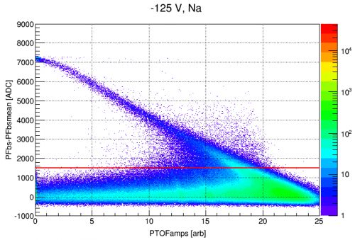
PuBe

Tail cut (Replaced by v2 of cBShi)
A cut on the baseline slope was also used to remove events on the tails of earlier pulses. To do this, the PT baseline change (PTdbs) was calculated by taking the sum of individual channel baseline changes (as measured by P*bs and P*bspost) weighted by the balancing factors used in constructing PT.

float bf[6] = {1.128, 1.323, 0.732, 1.24, 0.929, 0.647} // recommended balancing factors for -125 V data
z->SetAlias("PTdbs",Form("%e*(PAbspost-PAbs) + %e*(PBbspost-PBbs) + %e*(PCbspost-PCbs) + %e*(PDbspost-PDbs) + %e*(PEbspost-PEbs) + %e*(PFbspost-PFbs)",bf[0],bf[1],bf[2],bf[3],bf[4],bf[5]))

A simple cut was made using this quantity which identified events on a tail as those with a drop in PTbs larger (more negative) than 100 ADC. This roughly corresponds to a baseline change equal to the height of a ~100 eV PT pulse.

TCut ctail="PTdbs<-100"//Gives PT/dbs(1keV)~10

The cut line is shown below for each dataset in two energy ranges. Events below the line are removed. The x-axis is uncalibrated PTOFamps (there is a factor of 10^-6 hidden behind the color scale) but it the scale is roughly keV. The y-axis is the PTdbs quantity, which is a sum of scaled ADC units. The tails of large triggered events raise the ending baseline, hence the general trend of increasingly positive baseline change with energy. The events above the central band are pileup events which are almost entirely removed by later cuts (ofint and ofmax).

At low energies, all datasets tend toward downward-sloping baselines. In the bkg data, it is the most mild, with noise traces having an average PTdbs~-25. The Na data has much larger variation and comes in around PTdbs~-80 while the PuBe data has an average of PTdbs~-50 for noise traces. This is likely just a result of pulse pileup due to the higher event rate in the PuBe and Na datasets. Of the 3, the Na data will take the highest efficiency hit from this cut. However, the Optimal Filter can be biased by sloped baselines, so it is important to use the same selection criteria across the board here.

	~4 keV	~30 keV
Bkg
Na
PuBe

OF/INT consistency cut
v1:This cut was made to include only those events for which the single template Optimal Filter PT amplitude is consistent with the filtered PT integral. This will remove events which have pileup because INT measures all pulses in the traces while OF just fits one in the OF search window window. It can also remove events for which the OF is a poor fit due to excessive noise or a strongly sloped baseline.

TCut cofint_bkg = "PTINTall< (PTOFamps>12e-6)*9e6*(PTOFamps-12e-6)**2+178*PTOFamps+0.3e-4 && PTINTall>(PTOFamps>15e-6)*8.8e6*(PTOFamps-15e-6)**2+140*PTOFamps-1.5e-4"
TCut cofint_Na = "PTINTall< (PTOFamps>10e-6)*1.7e7*(PTOFamps-10e-6)**2+170*PTOFamps-0.2e-4 && PTINTall>(PTOFamps>15e-6)*1.5e7*(PTOFamps-15e-6)**2+135*PTOFamps-2.1e-4"
TCut cofint_PuBe = "PTINTall< (PTOFamps>10e-6)*1.2e7*(PTOFamps-10e-6)**2+170*PTOFamps+0.2e-4 && PTINTall>(PTOFamps>15e-6)*1.5e7*(PTOFamps-15e-6)**2+140*PTOFamps-2.1e-4"

At energies above ~20 keV, TES saturation becomes significant and the single template OF quantity also saturates. The 60 keV line is heavily saturated and can be seen at PTOFamps~30e-6. Some effort was made to include the beginning of this saturated region in the OF/INT cut, but it eventually cuts off these saturated events. An upper analysis threshold will need to be set due to this saturation.

	~4 keV	~30 keV
Bkg
Na
PuBe

v2:Each of these cuts were later divided into a pair defining events which had either too high of an INT/OF ratio or too low of an INT/OF ratio. This was done because events above the band are identified as pileup events, while those below have lowered INT quantities due to a sloped baseline.

TCut cofintHi_bkg = "PTINTall > (PTOFamps>12e-6)*9e6*(PTOFamps-12e-6)**2+178*PTOFamps+0.3e-4";
TCut cofintLo_bkg = "PTINTall < (PTOFamps>15e-6)*8.8e6*(PTOFamps-15e-6)**2+140*PTOFamps-1.5e-4";
TCut cofintHi_Na = "PTINTall > (PTOFamps>10e-6)*1.7e7*(PTOFamps-10e-6)**2+170*PTOFamps-0.2e-4";
TCut cofintLo_Na = "PTINTall <(PTOFamps>15e-6)*1.5e7*(PTOFamps-15e-6)**2+135*PTOFamps-2.1e-4";
TCut cofintHi_PuBe = "PTINTall > (PTOFamps>10e-6)*1.2e7*(PTOFamps-10e-6)**2+170*PTOFamps+0.2e-4";
TCut cofintLo_PuBe = "PTINTall <(PTOFamps>15e-6)*1.5e7*(PTOFamps-15e-6)**2+140*PTOFamps-2.1e-4";

v3: To make the cut less subjective, vertical slices of the INT-OF plane were fit with the crystal ball function. The slices were taken over 20 evenly spaced windows from PTOFamps = 0.1e-6 to 16e-6. Then points at mu+3*sigma from each fit were all fitted with the same empirical function used above for the earlier of-int cuts. The offset value was fixed at 1e-4 because the noise wall tended to make this fit parameter unstable. The resulting cuts identify events with relatively high OF/INT ratios. Note that these cuts make use of the bs and bs slope corrected INTall quantities defined in the corrections section below.

TCut cofintHi_bkg="PTINTall_PTdbscorr_bscorr> (PTOFamps>1.09042e-05)*6.21097e+06*(PTOFamps-1.09042e-05)**2+170.476*PTOFamps+1e-4"
TCut cofintHi_Na="PTINTall_PTdbscorr_bscorr> (PTOFamps>7.96642e-06)*1.22109e+07*(PTOFamps-7.96642e-06)**2+169.406*PTOFamps+1e-4"
TCut cofintHi_PuBe="PTINTall_PTdbscorr_bscorr> (PTOFamps>9.59954e-06)*1.22032e+07*(PTOFamps-9.59954e-06)**2+171.253*PTOFamps+1e-4"

The lower cuts have been removed in this version. Events which fall above the band are generally pileup, the trace integral being too large given the triggered pulse amplitude. Events below the band, however, are generally good pulses with the remnant of a small pulse tail in the prepulse. This gives an elevated bs, lowering the integral. These events have PFstd small enough to pass earlier cuts. However, they also come with elevated PTOFchisq, so should be removed by that cut if the prepulse variation is sufficiently severe.

OFdelay/WKr50 timing cuts
Two rough cuts are made on the pulse timing quantities PTOFdelay and PTWKr50. The first is to exclude events which have OFdelay values at the edge of the OF window. If there is a pulse partially outside the window, the OF delay and OFamplitudes will not be correct.

TCut cofdel="(PTOFdelay<23e-6 && PTOFdelay>-74e-6)"

A loose consistency cut is made on PTOFdelay and PTWKr50, the time of 50% rising edge of PT. This removes many noise events as well as otherwise good events with a pile-up pulse in the final few bins of the trace. These can leak through the OF-INT consistency cut. This cut is also needed to ensure PTWK is fitting the same pulse that OF is which is required for later glitch removal cuts. In the figures below, only events inside the 4 lines are retained.

TCut cofwktiming = "(PTOFdelay*1e6<PTWKr50*1e6-390 && PTOFdelay*1e6>PTWKr50*1e6-470)"

Bkg
Na
PuBe

The use of these timing cuts eliminates the need for the previously used OF-WKmax consistency cut as they were found to effectively remove all events which would have failed the OF-WKmax cut.

Glitch and Spikey Cuts
As discussed here, two populations of events were found when setting standard quality cuts. One type appears to be DCRC readout glitches. For these, it appears that a portion of the trace is from some other, unrelated place in the DCRC memory. The other type is a train of spikey pulses which were observed only in the first part of the n125V_PuBe data. Due to it's transience, this is assumed to be an unidentified noise source coupling to the electronics. Both of these populations are characterized fall times much faster than signals due to true phonon pulses. This provides a good quantity to use in removing them.

TCut cglitch = "1e6*(PTWKf20-PTWKr100)<12"
TCut cspikey = "1e6*(PTWKf20-PTWKr100)<35"

In the figures below, the glitch events appear as a band at PTWKf20-PTWKr100 ~ 7 μs and the spike train events at PTWKf20-PTWKr100 ~ 25 μs. The spikey events are most prominent in PuBe datasets 1 and 2, though there may be a sprinkling in the Na data as well. Events falling below the black and red lines fail the glitch and spikey cuts respectively, and are discarded from further analysis.

	~1 keV	~30 keV
Bkg
Na
PuBe Dataset 1,2
PuBe Dataset 3,4

OFchisq Cut
As described here, a cut was made on PTOFchisq to remove events which are poor fits to the template. In the figures below, all events above the red line are discarded. Note that the chisq is calculated in frequency space, so noise events will fail this cut if their spectrum is too different from that of the template (weighted by the average PSD).

TCut cchit = "PTOFchisq<(PTOFamps>6e-6)*((PTOFamps-6e-6)/3e-8)**2+PTOFamps/2e-9+5e3"

	~1 keV	~30 keV
Bkg
Na
PuBe

Low Energy Rate Cut
Note 52 and Note 55 describe the details of the Low Energy Rate Cut in -125V data.

The HV detector signal is expected to vary with parameters such as crystal temperature, detector bias, and TES bias point. While these are kept as stable as possible, some variations do occur. This section shows some attempts to use available data to infer variations in such quantities and make corrections based on those variations.

Baseline Correction

As explained here, pulse amplitude is expected to change with channel baseline. In order to correct for this effect, we need a consistent measure of baseline. This must be defined over several different time periods due to SQUID lockpoint jumps. The definition of this quantity is shown below for each of the 3 data types.

double bstime_bkg[]={1537.98e6, 1538.56e6, 1539e6}//Start times of the different PFbs periods
double bsmean_bkg[]={2742.5, 2707.5, 2112.5}//mean good baseline positions. 
z_bkg->SetAlias("PFbsmean",Form("(EventTime>%e&&EventTime<%e)*%e + (EventTime>%e&&EventTime<%e)*%e + (EventTime>%e)*%e",bstime_bkg[0],bstime_bkg[1],bsmean_bkg[0],bstime_bkg[1],bstime_bkg[2],bsmean_bkg[1],bstime_bkg[2],bsmean_bkg[2]))

double bstime_Na[]={1537.9e6, 1538.6e6, 1538.77e6}//Start times of the different PFbs periods
double bsmean_Na[]={3337.5, 3477.5, 2882.5}//mean good baseline positions. 
z_Na->SetAlias("PFbsmean",Form("(EventTime>%e&&EventTime<%e)*%e + (EventTime>%e&&EventTime<%e)*%e + (EventTime>%e)*%e",bstime_Na[0],bstime_Na[1],bsmean_Na[0],bstime_Na[1],bstime_Na[2],bsmean_Na[1],bstime_Na[2],bsmean_Na[2]))

double bstime_PuBe[]={1537.66e6, 1537.8e6, 1538.05e6, 1538.17e6, 1538.345e6, 1538.413e6, 1538.52e6}
double bsmean_PuBe[]={3100, 3220, 3260, 3860, 4740, 2700, 3260}
z->SetAlias("PFbsmean",Form("(EventTime>%e&&EventTime<%e)*%e + (EventTime>%e&&EventTime<%e)*%e + (EventTime>%e&&EventTime<%e)*%e + (EventTime>%e&&EventTime<%e)*%e + (EventTime>%e&&EventTime<%e)*%e + (EventTime>%e&&EventTime<%e)*%e + (EventTime>%e)*%e",bstime_PuBe[0],bstime_PuBe[1],bsmean_PuBe[0],bstime_PuBe[1],bstime_PuBe[2],bsmean_PuBe[1],bstime_PuBe[2],bstime_PuBe[3],bsmean_PuBe[2],bstime_PuBe[3],bstime_PuBe[4],bsmean_PuBe[3],bstime_PuBe[4],bstime_PuBe[5],bsmean_PuBe[4],bstime_PuBe[5],bstime_PuBe[6],bsmean_PuBe[5],bstime_PuBe[6],bsmean_PuBe[6]))

With this quantity defined, a simple linear correction can be made to remove most of this effect.

 z->SetAlias("PTOFamps_corr","PTOFamps*(1+3e-5*(PFbs-PFbsmean)")
 

This can also be done for the INTall quantity, after an initial bs slope correction (see next section below)

z_bkg->SetAlias("PTINTall_PTdbscorr_bscorr","PTINTall_PTdbscorr*(1.+0.18*(PFbs-PFbsmean)/2e3)")
z_Na->SetAlias("PTINTall_PTdbscorr_bscorr","PTINTall_PTdbscorr*(1.+0.22*(PFbs-PFbsmean)/2e3)")
z->SetAlias("PTINTall_PTdbscorr_bscorr","PTINTall_PTdbscorr*(1.+0.20*(PFbs-PFbsmean)/2e3)")

INTall bs slope Correction

The INTall quantity calculates the integral of the baseline-subtracted pulse. If a pulse is on a sloped baseline, the baseline will be over-subtracted, leaving much of the pulse negative and reducing the calculated integral. To correct for this, we can use the pre- and post- baseline rqs to infer the slope upon which the pulse is sitting and add a factor to the integral which adjusts for the “extra” area due to the sloped baseline. The figure below is an illustration of this idea. The pulse on an exponentially sloped baseline is shown in blue. It has been baseline subtraced so that the prepulse baseline is at 0. The orange shading shows the areas which contribute to the INTall quantity with those below the axis giving negative contribution. If the slope is large enough this results in a negative integral. The red line shows the correction factor suggested, it is simply the area of the triangle formed by the pre and post baselines and the trace length: (BSpre-BSpost)*4096. While this factor is not perfect, it can be a definite improvement on the standard INTall value.

For PTINTall, the correction uses the quantity “PTdbs”, the average baseline change of the 6 channels, weighted by their relative calibrations. The INTall corrected rq is defined as follows (the PAnorm factor is to convert PTdbs to ADC units):

z->SetAlias("PTINTall_PTdbscorr", "PTINTall-(PTdbs<0)*0.5*(PTdbs*4096./PAnorm)"

This correction factor will depend on the baseline slope/curvature, trace length, and the true pulse size and shape. For highly sloped baselines, such as in the model example shown above, the correction factor may be large. If the baseline is quite flat, it will be correspondingly small. As described, the correction is only sensible for pulses with a lower bspost than bs pre. The BSpost may be larger than BS pre if the bs there is a large pulse on a very flat BS (in which case no correction is needed) or if there is a pileup event late in the trace (which cannot be corrected for by this method).

An initial look at cut efficiencies can be found here

Further work comparing passage fractions to those expected from randoms is [Note 49], [Note 50], and [Note 58].

here, Note 52, and Note 55

Trigger Efficiency

Write Efficiency

Below is a version of our clean signal spectrum, along with background data scaled to the same livetime:

Figure 4.1
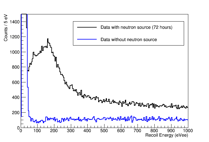72 raw hours of PuBe data. Background data scaled to the same livetime.

Figure 4.2 adds the n,gamma simulated signal

Figure 4.2

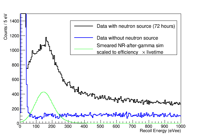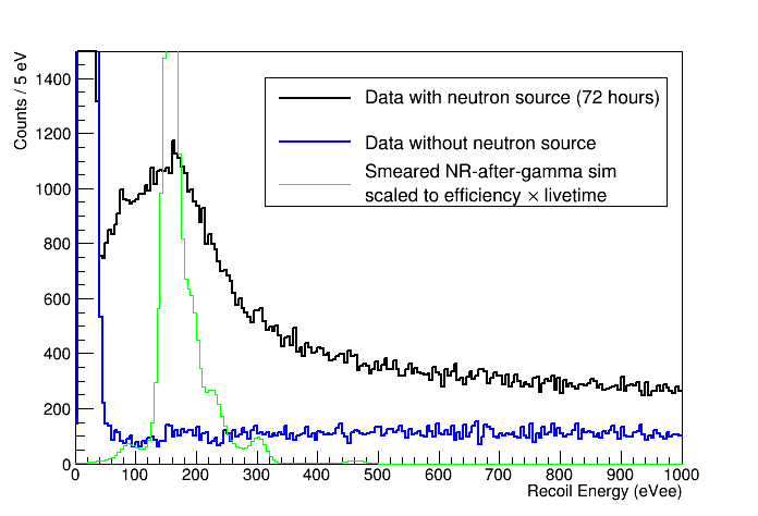
The simulated spectrum above has been energy-scaled and resolution-smeared by eye. Some notes:

• A yield of 0.2 was applied to approximately fit the data. This is close to Lindhard, which is about twice as high as previous measurements.
• A resolution of 50 eVee was applied, which smears out the individual peaks into what looks like a single gaussian.
• The normalization was done using 1) the measured Ge-70 capture rate 2) cross-sections and abundances of the other isotopes 3) livetime 4) all appropriate efficiencies (36% total)

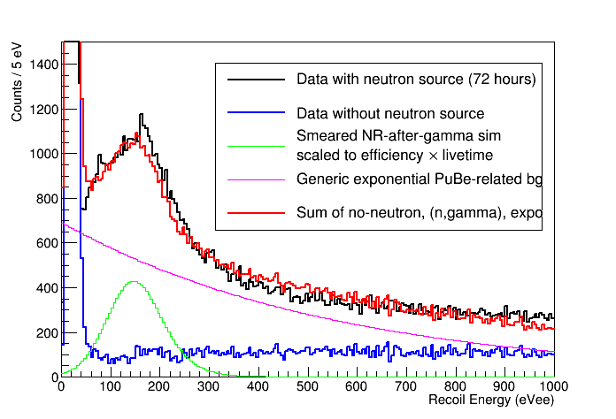
The normalization suggests that the size of our signal matches the simulation rather well. Below is a toy fit to show this better. Here I've subtracted both the background and the sim from the data, fit that spectrum to a simple exponential (representing the elastic neutron scatter background and whatever else), then added them all up again

Figure 4.3

There are a few tantalizing features in the signal spectrum, around 80 eVee, 160 eVee, and 300 eVee. Below I show the simulated spectrum with less smearing, or no smearing, with the data, and with a yield of 0.23 applied. Some of the peaks in the simulated spectrum seem to line up with the features in the data. (But to make the sim fit the data would apparently require some “hybrid” smearing.)

Figure 4.4
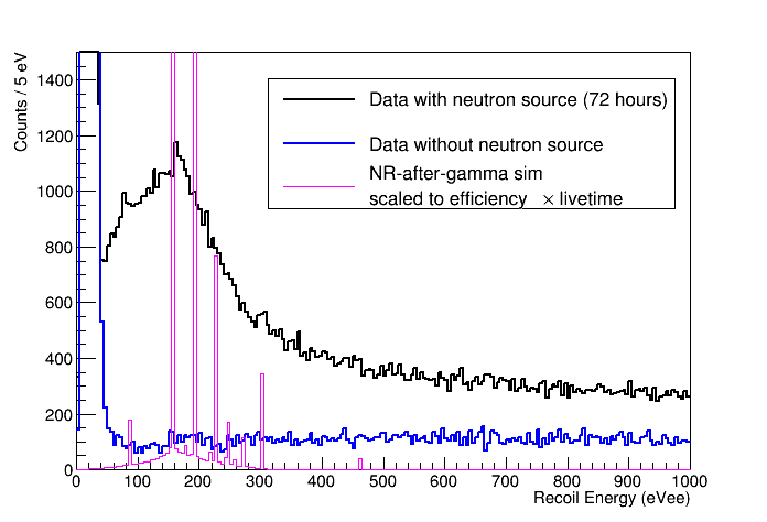Yield 0.23 applied to simulation. Some of the simulated peaks line up approximately with data.

Migdal Analysis

Full Signal Fit