R68 Trigger Efficiency

It is important to understand the efficiency with which our DAQ triggers on events as a function of event energy. Events with low energy may only sometimes satisfy the trigger condition due to random noise fluctuations. This effect may be important in R68, where much of our desired signal is just above the noise wall. This page contains information about studies to understand this effect.

One way to understand the trigger efficiency is to create fake pulses with the expected signal and noise spectra, pass them through a software simulation of the DCRC firmware trigger logic, and use study the triggering to understand the triggering efficiency as a function of fake pulse energy. A first pass at this was performed using a single PuBe series. The code is at: /home/mast/cdms/analysis/run068/trigger/r68_n125_trigger_sim.c

The steps taken are described briefly below.

1) Obtain a set of N prototype events at energies which should have 100% trigger efficiency. These will hopefully span the partitions space in a representative way. Let's select them from 0.5-1keV range. This results in a selection of N=52 events. The figure below shows the pF partition selection for these events.

pF vs energy for a single PuBe with prototype event region shaded

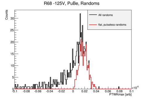
2) Select M good randoms (flat baseline, pulseless). These will be the noise instances into which we'll inject fake pulses. The selection criteria include high baseline cuts and pulse cuts via PTWKmax. These cuts result in the selection of M=326 good events from the 1000 randoms of a single PuBe series. The PTWKmax distribution of these events are shown in the figure below.

Selection of good randoms

3) Choose L=100 low energies from 0-0.5 keV that we'll simulate pulses at. For each of those M randoms, scale each of the N prototype event pulse amplitudes to each of the L low energies. Ideally this will give us the amplitudes that a lower energy event would have, if it was at the same location as the prototype event. Then use those scaled amplitudes to insert simulated pulses into the randoms using the OF templates. An example of such an event is shown below.

Simulated 250 eVee PuBe event

4) Run the trigger algorithm on all of these fake events using the same trigger conditions as in the real run (PA/PC/PF = 7/10/9 ADC). Obtain trigger efficiency vs. simulated event energy. For this preliminary study, only a subset of the LxMxN combinations were actually simulated due to computation time. The resulting trigger efficiency curve is shown below. The offset is the trigger efficiency calculated at 0 energy. In this simulation, it is the fraction of noise traces which meet the trigger condition. Putting better restrictions on the trigger times that count as triggering on the injected pulse would be more correct and lower this offset, but it shouldn't change the important factors of the energy at the step center, E0, and the step width, sigma. The 100% trigger efficiency below 60eVee indicates our assumption that 0.5-1 keV events were a reasonable selection of events with perfect trigger efficiency.

Preliminary trigger efficiency curve

The resulting curve is plausible. This result can be improved by repeating with higher statistics to better sample the channel partition space and variations in noise spectrum throughout the entire run. It should also be confirmed that the software trigger algorithm simulates the DCRC triggering by passing true DCRC triggered events through the algorithm. Another good check would be whether the rate of triggering on random traces (60%) is indeed consistent with the random trigger rates observed in data. Finally, we did take data with different trigger conditions, such as disabling one of the 3 triggering channels. It would be interesting to see if differences in the energy spectrum of those triggered events can be explained by corresponding simulated change in trigger efficiency.

The series used above was 07180922_2130, which was one of the first -125V PuBe series recorded. The above analysis was later repeated with a different series from the middle of the PuBe data to understand the stability of the trigger efficiency. The series used here was 07180924_1710, the first series from dataset n125_PuBe_2.

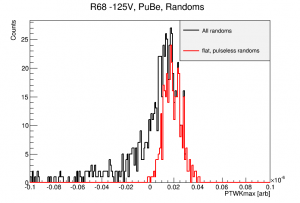Trigger simulation plots for 07180924_1710

The resulting trigger efficiency curve is quite different. It starts at a higher value (indicating more triggering on noise), reaches 100% at a higher energy, and is not monotonic. The first two points can simply be a result of increased baseline noise.

The decrease in efficiency from 20 eV to 25 eV is also a result of triggering on noise. In some instances, a noise fluctuation near the trigger time can pass the trigger threshold. Then, if the noise phase is opposite that of the injected pulse, including the pulse at a similar amplitude can diminish the offending noise fluctuation so the combined trace no longer triggers. For still larger pulse amplitudes, it will again trigger on the pulse. This should be a rare occurrence, but in the above simulation, where only 34 sample randoms were used, it can affect the final efficiency curve.

If we restrict the noise traces used to those which do not trigger without a pulse, we obtain a smoother looking trigger efficiency. However, we have to think carefully about how we may be biasing this result by using only the least-noisy traces.

Trigger efficiency curve for 07180924_1710	+ without using noise traces which trigger.

Due to computational time, the simulations above used only 10% of the suitable random traces (M values). Assuming such cases as outlined in the figure above are rare, such fluctuations should smooth out with more statistics. This is borne out in the curves below where the trigger simulations were carried out using the full set of 349 good randoms, 69 good prototype events, and 25 energy bins. The result is a smooth trigger efficiency curve, though the result no longer follows the sigmoid model. Instead we use an exponential model with offset. The offset at 0 energy is again interpreted as related to the noise trigger rate, and the remaining rise as the trigger efficiency curve.

Higher stats simulation for 07180924_1710

These higher stats simulations were completed for several series throughout the PuBe data. In particular, the first series from each n125_PuBe* dataset, and the final series were simulated. The fraction of triggering events and inferred trigger efficiencies are shown below. Variation in these curves are generally similar. This is consistent with the stability of noise distributions studied elsewhere.

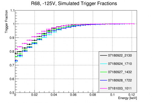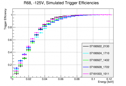Results of trigger efficiency simulations for several series throughout the PuBe dataset.

Each of these curves was fit with the simple empirical model,

.

The distribution of fit parameters gave, <E_0> = 30.86 eVee and stdev(E_0) = 2.05 eVee. The average fit and region spanned by the 3σ range of the fit parameter, E_0, are shown on the figure below. This defines the final, recommended trigger efficiency for use in Run68 PuBe data.

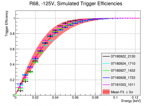Fitted simulated trigger efficiency function

Above, quality cuts were used to select flat, pulse-less randoms. However, this could introduce a bias as low energy events may be less likely to trigger on sloped traces. We want to know the likelihood of an event which occurs at a random time to issue a trigger, regardless of the state of the detector channels. To do this, we should not use any quality cuts when selecting randoms. Otherwise, the rest of the procedure for simulating and calculating the efficiencies is as described above.

The resulting trigger efficiency curves are shown below. This analysis uses variable width binning to extend to 1keV without making computation prohibitively expensive. The points are spaced by 10 eVee from 0 to 300 eVee, then by 50 eVee up to 1 keVee. Instead of fitting to an empirical model, we instead will use the average binned efficiencies in the final R68 analysis. The uncertainty of the efficiency was calculated as the standard deviation of the 5 simulated efficiencies. This systematic dominates the statistical uncertainties below 0.75 keV. Above that point, the statistical uncertainties dominate, but are at the 10^-3 level.

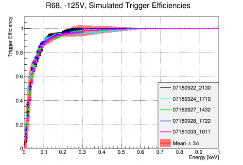Simulated Trigger Efficiencies with no pre-selection of noise traces