Table of Contents
R68 -125V Full Signal Fit
Methods
This describes how we fit the final measured spectrum, with all quality cuts included, to the total simulated spectrum. The goal of this fitting is to extract an estimate of the nuclear recoil yield in the range of energies near the (n,gamma) capture signal. This analysis was done in the python notebook located at:
/home/mast/cdms/analysis/run068/simulations/k100_ncapture_cal/R68_Y_fit.ipynb
Data Sets
The final measured event spectra were determined using the cuts and calibrations described here. The individual event energies for PuBe and Bkg datasets were exported to the following text files:
/home/mast/cdms/analysis/run068/simulations/k100_ncapture_cal/data/r68_n125_PuBe_cgood_final_PTOFkeV_2keV_scan_fmt.txt
/home/mast/cdms/analysis/run068/simulations/k100_ncapture_cal/data/r68_n125_bkg_cgood_final_PTOFkeV_2keV_scan_fmt.txt
The simulated Geant4 output files are:
/data/chocula/villaa/k100Sim_Data/captureCal/Run68_gdirect_bknd_R68_PuBe_0x0006_10M_155*.txt
These files contain many interactions of many types both in and outside of the detector. Skims were made of these files to select out appropriate interactions in the HV detector. Some of these 40261 G4 output files are incomplete (missing lines, values, etc.) These are simply skipped in the skim and leave 39329 files which were actually included. The skims used are located at:
data/home/mast/cdms/analysis/run068/simulations/k100_ncapture_cal/data/
The two skims used in this analysis are:
R68_gdirect_testskim_stupidhighstat_nocap_nr.h5
R68_gdirect_testskim_stupidighstat_nocap_er_lowe.h5
the first of which includes nuclear recoils, but no capture events the other which has only electron recoils below 10 keV.
The simulated (n,gamma) cascade events are taken from the file:
/data/chocula/villaa/cascadeSimData/normsi_Quant_fast.pkl
From Simulated Hits to Measured Energy
In general, the outputs of the simulation are individual interactions in the detector and we have to do some work to construct a measured energy estimate from them. The general steps followed for each type of data are shown below.
ER
For an incoming gamma, energy is deposited in the detector material both directly and by ionizing electrons which then deposit their energy. Since yield is not an issue for these events, we can simply sum up all the hits and treat the total energy. The steps to calculate measured energy from ERs are as follows:
- Sum deposited hit energies to get total recoil energy, E_recoil
- Apply Fano factor to total recoil energy
- Calculate Eee = E_recoil since we calibrate to E_recoil.
- Apply detector resolution function (w/o Fano contribution) to E_ee.
NR
The NRs are handled differently. Typically, the hits that appear in the G4 output are a Si nucleus starting with some energy, which it deposits in a single step. About 99% of the NR events consist of <5 such hits. The yield and Fano factor should be applied to each recoiling nucleus independently before summing to total measured energy.
- Use Yield to calculate Ionization energy deposited from each hit: N = Y(E_recoil)*E_recoil/ε
- Apply Fano factor to each hit
- Calculate E_tot = N*V + E_recoil for each hit
- Sum E_tot from hits to form each event
- Convert to E_ee = E_tot/(1+V/eps)
- Apply detector resolution function (w/o Fano contribution) to E_ee.
(n,gamma)
From Anthony's notebook SiCaptureSpectrum.ipynb: “Since the capture events consist mostly of composite nuclear recoils, we must decide how to account for the ionization yield correctly for each cascade step. Assume a nuclear recoil created by a cascade step begins at energy and deposits energy
in the step. We would then expect the ionization to be that which would have been given from a deposited energy of
less that which would have been given from a deposit of
. This simply assumes that the ionization is independent of the slowing-down history of the particle, or, that any recoil of energy
will give a reproducible amount of ionization regardless of the circumstances of its creation.”
This means that the amount of ionization energy in a given step, i, is
and the total number created in an event is simply:
Similarly, we will assume that the variance of each step is: , where
is a nuclear recoil Fano Factor. If we further assume the hits are uncorrelated the total variance of the event is
so that, for an energy-independent Fano factor, we have
.
- Get N for each step
- Apply F_NR to each step
- Calculate E_tot = N*V + dE_recoil for each step
- Sum E_tot over the whole event
- Convert to E_ee = E_tot/(1+V/eps)
- Apply detector resolution function (w/o Fano contribution) to E_ee.
Mixed ER/NR
As described here, there are a small number (<1%) of events which have both ER and NR hits. The NR hits were generally <5 eVee, and so treating the ER and NR portions as separate events (as we did when generating the data skims) is incorrect, but should not have a noticeable effect on the final spectrum. The NR hits are below threshold and the amount by which the ER hits would be shifted by including the NR portion would be small.
Detector Resolution
The detector resolution was studied here. The observed total resolution was determined to be
with =10.27 eV and B=0.627*3.8 eV. This was determined by fitting the distribution of widths of ER calibration peaks, so part of B is due to Fano statistics. As described above, we treat the Fano part before applying detector resolution. So the detector response, without Fano, uses instead
.
Averaged Spectra
When generating complete spectra using the steps above, there are 2 ways to handle the smearing effects of Fano and detector resolution. The first is to generate a single realization of the measured energy while the second is to construct the averaged spectrum straight away. In the single realization, we select a discrete number of e-/h+ for each hit by selecting it from the Gaussian/Fano PDF and then select a single value from the Eee distribution set by the detector resolution function. Then all such values in the dataset are histogrammed to form the spectrum. Thus a single event will result in a single count in one bin of the final histogram, and such a histogram represents a single realization of the spectrum. We can then construct many such histograms and average them to get the average expected distribution. The other option is to generate the average spectrum in one pass. This is done by choosing the final Eee histogram bins from the outset and filling the bins not with discrete counts, but according to the probability distributions of each event. To do this, we calculate <Eee> and sigma_ee for each event and fill the histogram with the appropriate values integrated from the Gaussian/Fano distribution. This is done for each event and the resulting spectrum is the average Eee spectrum. After it is constructed, this spectrum is smeared with the detector resolution function to produce the final, averaged Eee spectrum.
The mean, electron-equivalent energy, for a recoil of energy Er is calculated as
and, as described here, the width in units of Eee is
where E_ion = Y*Er and Y=1 for ERs, Y=Y(Er) for NRs, and F is the ER or NR Fano factor as appropriate.
These two methods have been shown to be equivalent by generating many single spectrum realizations and comparing their average to the result of average spectrum method.
Note one expected difference is the way hits with are handled. When simulating a single instance of such a hit (i.e. in `buildSpectra`), we use the function `getNeh` to draw a discrete number of e/h pairs from a normal distribution, with values <0 disallowed. However, in the `buildAvgSpectra` function, we don't round or implement that hard cutoff, i.e. the distribution of possible amplitudes may have a substantial tail below 0 energy for depositions near 0.
Timing
Note, there are still some hits in some 'EV' which are well separated in time. These should eventually be split into separate events.
Yield Models
Lindhard, parameterized in Lewin and Smith
Nuclear Recoil Fano Factor
Could be O(1): Dougherty
Efficiencies and Live Time
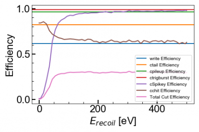
Our best estimates of several energy-independent cut efficiencies are applied to the final simulated spectra. The simulated trigger efficiency, Spike Cut Efficiency, and Chisq Cut Efficiency are also applied and all have energy dependence which pulls down the low energy rates. The DAQ write efficiency was 61.7% on average for PuBe data.
 |
The livetime of measured data is calculated from the time between the first and last triggered event of each series.
| Data | LiveTime |
|---|---|
| Bkg | 24.1 |
| PuBe | 97.9 hr |
The Geant4 simulation data is all generated by throwing primaries from the PuBe source. We can understand the simulated livetime by matching the simulated captures to the observed Ge-70 capture rate in a Ge HV detector in Run66. From that, Matt made the following calculations:
| Measured | isotopic fraction | x-section (bn) | Rcapture (1/s) |
|---|---|---|---|
| Ge-70 | 21% | 3.4 | 1.38 |
| Ge total | 100% | - | 4.55 |
| Predicted | isotopic fraction | x-section (bn) | Rcapture (1/s) |
|---|---|---|---|
| Si-28 | 92% | 0.08 | 0.161 |
| Si-29 | 5% | 0.28 | 0.031 |
| Si-30 | 3% | 0.4 | 0.026 |
| Si total | 100% | - | 0.218 |
These rates assume detectors of equal size and account for the relative number density of Si and Ge. For Run 68 the relevant number is the total capture rate on all isotopes in the silicon detector: 0.218 captures/second. So for the (n,gamma) sim, the total number of events divided by 0.218 gives the simulation time in seconds. For the GEANT sim, we count the total number of captures and divide by 0.218 1/s.
| Simulation | File | Event Count | Simulated Livetime (hr) |
|---|---|---|---|
| G4 PuBe | k100_ncapture_cal/data/R68_gdirect_testskim_stupidhighstat_wcap.h5 | 14844 captures | 18.9 |
| (n,gamma) | /data/chocula/villaa/cascadeSimData/normsi_Quant_fast.pkl | 200,000 cascades | 255 |
N.B. The files “R68_gdirect_testskim_stupidhighstat_*.h5” were produced using the flag: ```–regex 'Run68_gdirect_bknd_R68_PuBe_0x0006_10M_155\\S+.txt'``` with the sima2py in the git hash: f0c2a47. These skims use the full set of 40261 G4 output files. The resulting skims are located in /home/mast/cdms/analysis/run068/simulations/k100_ncapture_cal/data/ . Some of the 40261 G4 output files are incomplete (missing lines, values, etc.) These are simply skipped in the skim. There are 932 such files as can be seen by counting the 'Incomplete' labels in the output of sima2py, such as in the file R68_gdirect_testskim_stupidhighstat_nocap_er_lowe_skimfiles.txt. This leaves 39329 files which were actually included. Each file was from a simulation which threw 10M n's. Given the estimated PuBe n rate of (2.28 ± 0.06)E6 n/s, each file represents a livetime of 4.39±0.12 s and the stupidhighstat skims represent (48.0 ± 1.3) hr of livetime.
Results
MCMC Fitting
Preliminary
An example of the generated spectra using the Damic yield function is shown below. The overall normalization of the smulated ER+NR spectrum was set to match the measured spectrum from 1-2 keV. While the continuum spectrum can be made to agree above 300 eVee, the capture component is clearly too low and there is disagreement below 100eVee.
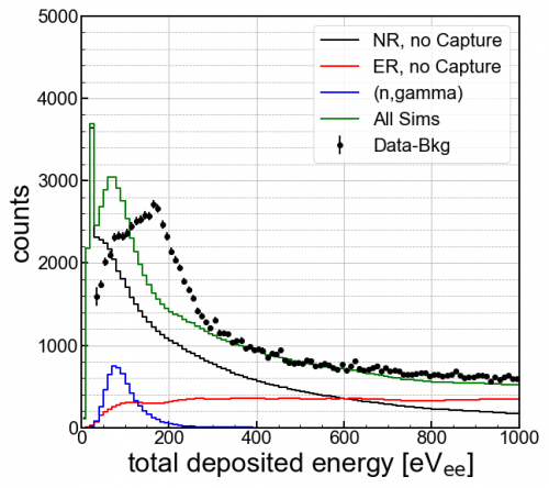 |
| Spectra comparison using Damic Yield function |
|---|
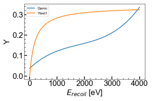
In this figure, a crude parameteried yield model has been used to move the capture peak closer to its observed position. The yield at that point is more than twice that which Damic measured and F_NR=1. This model still shows disagreement below 100eVee.
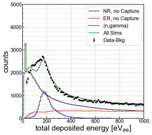 |  |
| Example spectrum with simple parameterized yield model | |
|---|---|
However, removing the detector resolution seems to give a better fit and no low-energy spike in the NRs. It is difficult to see how resolution smearing could plausibly produce this spike. This is currently under investigation.
This spike also appears slightly differently for the two spectrum methods. This could depend on the difference in how low energy Fano is applied.
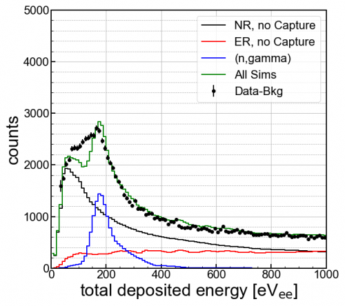 |
| Parameterized Yield model with no detector resolution |
|---|
Now a few improvements have been made. The source of the spike above was the incorrect order of trigger efficiency and detector resolution. The estimated livetimes have also been included so we can compare rates. The figure below still uses a non-standard yield parameterization, uses F_NR=2.1, and requires scaling up of simulated signals by 1.5. Detector resolution is applied here.
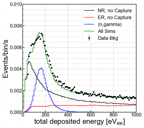 |
| Improved spectrum with funny yield model and detector resolution |
|---|