Table of Contents
Calibration and Resolution
Am-241 spectrum reference paper
Summary
This section gives lines of code for the latest, best calibrations. The calibration varies between the three datasets: -125V Background, -125V Na, -125V PuBe.
In the code below it is assumed you have loaded the data into a TChain called “z”.
These calibrations convert amplitude PTOFamps into keVee. They are only accurate with the appropriate cuts applied, i.e. they are unlikely to be correct for tails, pileup, or retrigger events.
-125 V Background Data Calibration
First, apply Nick's baseline correction:
double bstime_bkg[]={1537.98e6, 1538.56e6, 1539e6}//Start times of the different PFbs periods
double bsmean_bkg[]={2742.5, 2707.5, 2112.5}//mean good baseline positions.
z->SetAlias("PFbsmean",Form("(EventTime>%e&&EventTime<%e)*%e + (EventTime>%e&&EventTime<%e)*%e + (EventTime>%e)*%e", bstime_bkg[0], bstime_bkg[1], bsmean_bkg[0], bstime_bkg[1], bstime_bkg[2], bsmean_bkg[1], bstime_bkg[2], bsmean_bkg[2]))
z->SetAlias("PTOFamps_corr","PTOFamps*(1+3e-5*(PFbs-PFbsmean))")
Next, set a correction factor for the observed shift of the calibration between the two parts of the background data:
z->SetAlias("cfac","1+(SeriesNumber<71809280000)*0.010333")
The final calibration is
z->SetAlias("PTOFkeV","8.068258e+05*PTOFamps_corr*cfac+1.901617e+10*(PTOFamps_corr*cfac)**2");
-125 V Na Data Calibration
First, apply Nick's baseline correction:
double bstime_Na[]={1537.9e6, 1538.6e6, 1538.77e6}//Start times of the different PFbs periods
double bsmean_Na[]={3337.5, 3477.5, 2882.5}//mean good baseline positions.
z_Na->SetAlias("PFbsmean",Form("(EventTime>%e&&EventTime<%e)*%e + (EventTime>%e&&EventTime<%e)*%e + (EventTime>%e)*%e",bstime_Na[0],bstime_Na[1],bsmean_Na[0],bstime_Na[1],bstime_Na[2],bsmean_Na[1],bstime_Na[2],bsmean_Na[2]))
z->SetAlias("PTOFamps_corr","PTOFamps*(1+3e-5*(PFbs-PFbsmean))")
Next, set a correction factor for the observed shift of the calibration between the two parts of the Na data:
z->SetAlias("cfac","1+(SeriesNumber<71810000000)*0.012")
The final calibration is
z->SetAlias("PTOFkeV","6.822255e+05*PTOFamps_corr*cfac+3.089717e+10*(PTOFamps_corr*cfac)**2");
-125 V PuBe Data Calibration
First, apply Nick's baseline correction:
double bstime_PuBe[]={1537.66e6, 1537.8e6, 1538.05e6, 1538.17e6, 1538.345e6, 1538.413e6, 1538.52e6}
double bsmean_PuBe[]={3100, 3220, 3260, 3860, 4740, 2700, 3260}
z->SetAlias("PFbsmean",Form("(EventTime>%e&&EventTime<%e)*%e + (EventTime>%e&&EventTime<%e)*%e + (EventTime>%e&&EventTime<%e)*%e + (EventTime>%e&&EventTime<%e)*%e + (EventTime>%e&&EventTime<%e)*%e + (EventTime>%e&&EventTime<%e)*%e + (EventTime>%e)*%e",bstime_PuBe[0],bstime_PuBe[1],bsmean_PuBe[0],bstime_PuBe[1],bstime_PuBe[2],bsmean_PuBe[1],bstime_PuBe[2],bstime_PuBe[3],bsmean_PuBe[2],bstime_PuBe[3],bstime_PuBe[4],bsmean_PuBe[3],bstime_PuBe[4],bstime_PuBe[5],bsmean_PuBe[4],bstime_PuBe[5],bstime_PuBe[6],bsmean_PuBe[5],bstime_PuBe[6],bsmean_PuBe[6]))
z->SetAlias("PTOFamps_corr","PTOFamps*(1+3e-5*(PFbs-PFbsmean))")
Next, set a correction factor for the observed shift of the calibration in the middle period of the PuBe data:
z->SetAlias("cfac","1+(SeriesNumber>71809240000&&SeriesNumber<71810020000)*0.030125")
The final calibration is
z->SetAlias("PTOFkeV","7.278458e+05*PTOFamps_corr*cfac+2.651263e+10*(PTOFamps_corr*cfac)**2");
Calibration Lines in -125V Background Data (Am-241 and others)
Calibration shift, and correction
The -125V background data is comprised of two datasets separated by several days: n125_bkg_1 which ended on 2018 Sep 27 and n125_bkg_2 which began on 2018 Oct 03. The only intentional change between these times was the setup of the NaI detectors, so in principle there should be no difference. However a small but noticeable shift in the calibration appears between the datasets.
| Figure 1.1 | |
|---|---|
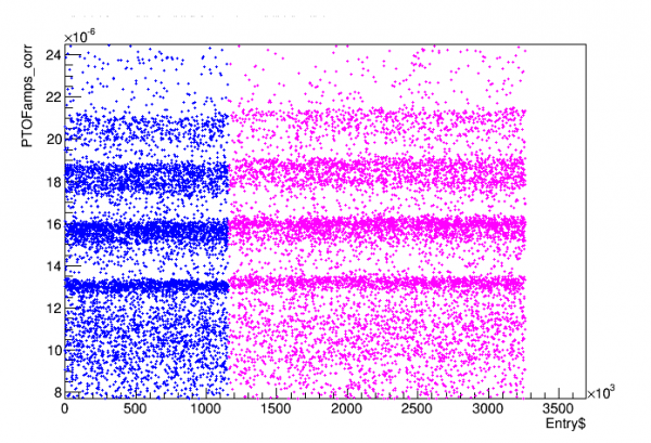 | 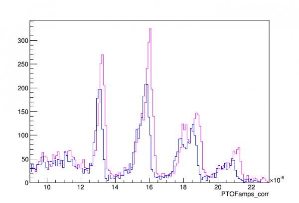 |
| Blue: dataset n125_bkg_1, Magenta: dataset n125_bkg_2 | |
note: PTOFamps_corr applies Nick's baseline correction to improve resolution.
I decided to combine all the data after applying a correction to match the two datasets:
// PTOFamps correction factor:
z->SetAlias("cfac","1+(SeriesNumber<71809280000)*0.010333")
// this factor can be multiplied by OF rqs as a correction, e.g.: PTOFamps*cfac, or PTOFamps_corr*cfac
| Figure 1.2 |
|---|
 |
| Combined data. Red: no correction. Green: with correction. |
Identified lines: Am, Pb, Au(!) (and Ag and Pd)
The data below is based on PTOF_corr with the time-based correction above. I use all of Nick's recommended cuts. To see the Am lines clearly I use a pF selection cut. It is a non-flat cut written by Nick and modified slightly:
// Nick's non-flat high-pF cut:
TCut cF = "PFOFamps/PTOFamps>0.5-PTOFamps*(0.5-0.22)/(20e-6)"
// here's a modification
TCut cFh = "PFOFamps/PTOFamps>0.28"
cF+=cFh
A standard calibration was performed (fitting the 14keV and 18keV lines and fitting a quadratic to these points and the origin). To identify features I used published energies and relative amplitudes of Am-241 lines and Pb x-rays (produced by the lead collimator). I also used a Geant simulation of the Compton spectrum from 60keV gammas on a Si detector. The simulation was roughly fit to data by 1) applying a scale factor 2) adding a flat backgkoooround 3) convolving with a Gaussian resolution of width 250 eV, approximately the same as the 14keV line width.
| Figure 2.1 | |
|---|---|
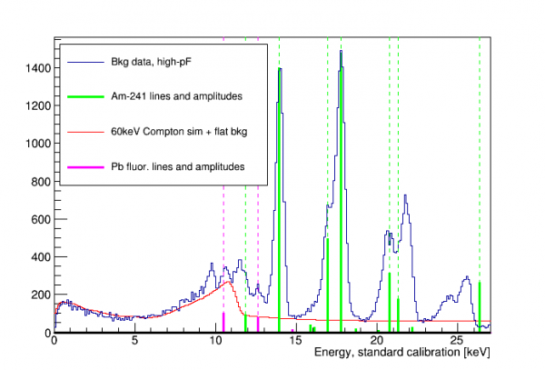 |  |
| The heights of the thick solid lines indicate relative amplitudes, scaled to the height of visible lines. Zooming in on lower energies (right) the 11.9keV Am line looks like a shoulder on another peak so there seem to be TWO unidentified peaks, around 9.6keV and 11.4keV |
|
Doing a brief search for the two unidentified lines at 9.6 and 11.4 keV suggested x-rays from gold. The Wikipedia article on Am-241 for smoke detectors states that, indeed, gold is used in the manufacture; there is actually a layer of gold on top of the AmO2. So looks like we've identified these lines!
| Figure 2.2 | |
|---|---|
 |  |
UPDATE: The unidentified lines above 20 keV correspond to silver and palladium x-rays. These elements are also listed as a part of smoke-detector Am source manufacture.
| Figure 2.3 |
|---|
 |
Lack of low-energy lines
The same reference with the L-shell Am lines and branching fractions also lists M-shell lines and amplitudes with the same relative amplitude scale. If we plot those along with the other lines it's clear that we should see them too, if they are getting to the detector:
| Figure 2.4 |
|---|
 |
If the relative amplitudes are correct then it appears that less than 5% of the x-rays around 3.5 keV are getting through to the detector. As noted in the 2016 Dec 30 run diary there is (should be) Kapton tape covering the collimator hole, intended to block alphas but not low-energy x-ray calibration lines. Given a chemical formula and density for Kapton – C22H10N2O5, 1.43 g/cm^3 – we can use the CXRO LBL calculator to find attenuation coefficients: for 3.5, 11.9, 13.9 keV we find 93, 4000, 6200 um.
| Table 2.1 | |||||
|---|---|---|---|---|---|
| Transmission | |||||
| Energy [keV] | Attenuation coeff. [μm] | 4 mil | 8 mil | 12 mil | 16 mil |
| 3.5 | 93 | 33.5% | 11.2% | 3.8% | 1.3% |
| 11.9 | 4000 | 97.5% | 95.0% | 92.7% | 90.3% |
| 13.9 | 6200 | 98.4% | 96.8% | 95.2% | 93.7% |
A single 4-mil layer of Kapton would still let a lot of the low lines through, but 16 mil could explain why the 3.5 keV line is not seen and the next higher lines are seen. (Alternatively it could be that the gold layer or something in the source is too thick to pass the 3.5 keV x-rays - but this seems unlikely since the source is designed to emit alphas.)
UPDATE: it's very possible that the source construction does not allow the low x-rays to escape the source itself. Various sources state that the source is a film of AmO2 mixed with gold, with an upper layer of gold or palladium and a lower layer of silver. The ORNL report (link in next section) describes typical thicknesses of 2 μm for the AmO2/Au layer, 1-2 μm for the upper layer, and 200 μm for the lower Ag layer. Given the source diameter and presumed 1 μCi activity (this seems to be standard for modern smoke detectors), this would imply a very small AmO2-to-Au ratio in the active layer, about 1.5 parts per thousand AmO2. So that layer is mostly gold.
If these dimensions are correct it would suggest that alphas should be able to escape the active layer and penetrate the upper layer, and are well blocked by the lower level. So this makes sense design-wise. (Also a 4 mil Kapton layer would block almost all alphas.)
As for x-rays, at 14keV the AmO2/Au layer would absorb about 25% of them. Combined with a 2 μm Pd outer layer and 4 mil of Kapton about 30% are absorbed. At 3 keV, only 12% escape the AmO2/Au layer, only 4% make it through a 2 μm Pd outer layer, and only 1% make it all the way through a 4 mil Kapton layer. If we cut both the AmO2 and Pd layer thicknesses in half we wind up with about 8% of 3keV x-rays penetrating.
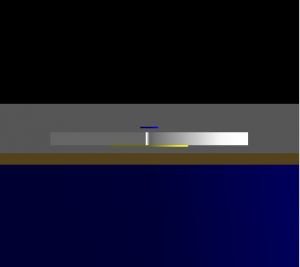
For the Geant4 K100 sim, in addition to the lead collimator I added an Am source with a 1.5 um thick gold middle layer, a 2 um thick palladium upper layer, and a 200 um thick silver backing. I also added a 4 mil thick layer of Kapton over the collimator hole. I threw 10 million each 60 keV, 14 keV, and 3.5 keV gammas from the middle layer. At 14keV there were 17955 full-energy hits in the detector. At 3.5 keV there were only 37 hits. So this is a stronger relative attenuation than what was estimated above: only 0.002 times as many 3.5 keV x-rays hit the detector as do 14 keV x-rays.
| Figure 2.5 | |||
|---|---|---|---|
 |  |  |  |
Different radial position selections
All the features in the previous section are associated with the Am source and thus show up best when a pF (low-radius) selection is applied. I also wrote a cut to select high-radius events:
TCut couter = "(PAOFamps+PBOFamps)/PTOFamps>0.255"
We can define three categories: Low-Radius (selecting high pF events), High-Radius (applying couter), and Mid-Radius (everything else). Below I look at spectra from all three radial categories to look for hints of lines that aren't restricted to low radii.
| Figure 3.1 | |
|---|---|
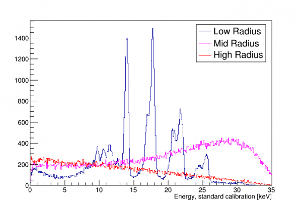 | 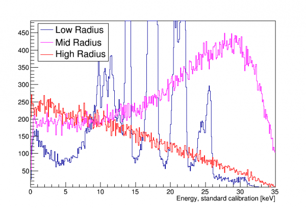 |
There's no strong evidence of lines in the mid- and high-radius selections. There may be a hint of the 8 keV copper fluorescence in the high-radius case, which would make sense because there's a lot of outer-wall copper. It's energy looks a little low which could be from reduced charge collection at high radius from field fringing. The plots below try to show this possible peak in other ways.
| Figure 3.2 | |
|---|---|
 |  |
The arrangement of the Am source (some details of the bare smoke-detector Am source here) should explain why all spectral features related to the source (direct and fluorescence of other materials) appear only in the center channels. Simulations were formed with the lead collimator and source dimensions, one simulation for 60keV gammas and another for 14keV x-rays. (Some details about how the Am source is manufactured can be found on Page 6 of this ORNL report on radioactivity in smoke detectors, or 3-13 of this NRC report.)
| Figure 3.3 | ||
|---|---|---|
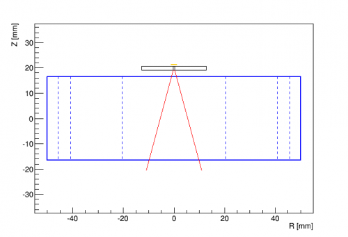 |  |  |
| Source and collimator arrangement | Red lines represent contours at 50% (z,r = 5.3,3.7 mm) and 90% (z,r = 21,11 mm) | Red lines represent contours at 50% (z,r = 0.4,1.4 mm) and 90% (z,r = 1.1,2.0 mm) |
Also seen in the 60 keV plot above (which selects energies between 6 and 12 keV) are shallow events at high radius. These are electrons scattered from the collimator, with energies from 0 to around 45 keV, probably from photoelectric absorption. Of the hits in the simulation, about 82% are full-energy 60keV events, and 2% are these surface events. Most of the rest are Compton scatters.
| Figure 3.5 |
|---|
 |
Because the calibration lines occur in pF, it's worth asking whether the other channels are even necessary to produce a sharp spectrum. Below is a spectrum of only the pF OF amplitude. It's clear that the resolution is much worse, so the energy in the other channels is indeed relevant.
| Figure 3.6 |
|---|
 |
| A spectrum based on only pF OF amplitude, rather than PT |
Below are some plots exploring position reconstruction. First below is a diagram of the channel layout for Side 1 (left side):
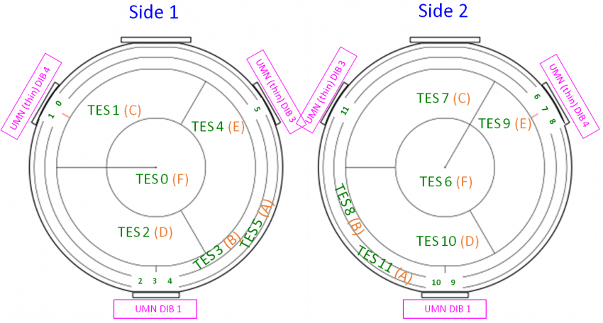
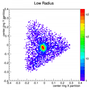
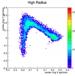
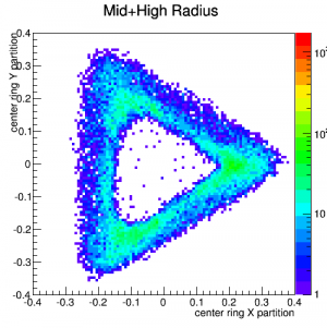
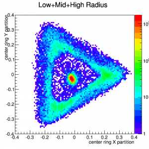
X and Y “partition” quantities were constructed using only the weighted amplitudes in the inner-ring channels C,D,E, and “triangle plots” were made for events from 13-19 keV (where the calibration peaks are) separately for low-radius, mid-radius, and high-radius events.
| Figure 3.7 | ||||
|---|---|---|---|---|
| x-y plots based on partitioning between the central ring channels, 13 -19 keV | ||||
 |  |  |  |  |
Below the same is done for X and Y “delay” quantities based on the relative timing between the inner-ring channels.
| Figure 3.8 | ||||
|---|---|---|---|---|
| x-y plots based on WKr30 time differences (delay) between the central ring channels, 13-19 keV | ||||
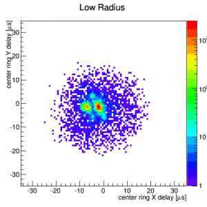 | 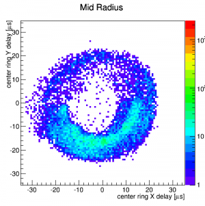 | 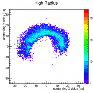 |  | 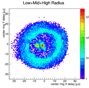 |
Splitting in the central peak is caused by the same pulse time glitch seen early in the run. This glitch caused us to switch to 10-minute runs, which reduced the problem in pF. It does not seem to strongly affect PTOF for pF events - but it may be hurting the resolution of events in other channels, where the glitch is more frequent. It would be difficult to tell since all our lines are in pF.
There is a clear asymmetry above: events in the upper half (y>0) seem to be “high radius” and events in the lower half seem to be “mid radius”. I re-did these plots with a different radial selection, where the radius cuts are based only on the center and outer-ring channels A,B,F. Results are here, and they are similar. I think this rules out the possibility that the asymmetry is due to an imbalance in the inner-ring channel gains.
Hence high-y events seem to share more of their energy with the outer rings than do low-y events.
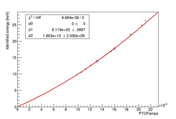
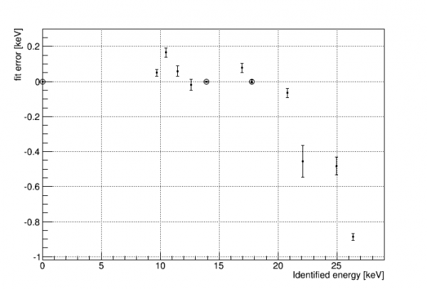
Calibration Curves
| Figure 4.1 | |
|---|---|
| Standard calibration (quadratic through 14keV and 18keV lines constrained to 0,0) | |
 |  |
| Figure 4.2 | |
|---|---|
| Full-range calibration (quadratic through all lines and constrained to 0,0) | |
 |  |
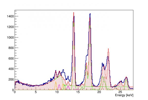
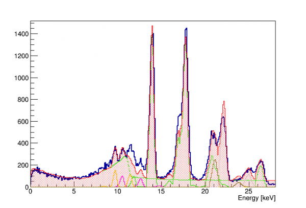
Based on the residuals in Figure 4.1 above an alternative calibration was created to fit both low and high energies, by adding to the quadratic a 1/x^n-type function with an asymptote near the saturation point. Below is a resulting full-range spectrum:
| Figure 4.3 |
|---|
| |
| Figure 4.4 | |
|---|---|
| Fit using resolution curve and published branching ratios: | Using asymmetrical peaks: LHS width = 1.5*RHS width: |
 |  |
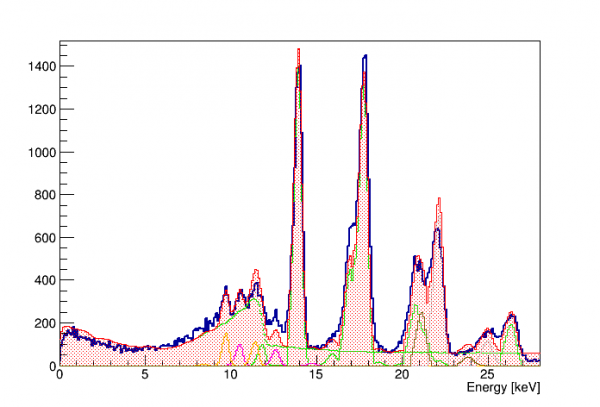
| Figure 4.5 |
|---|
| Adding an arbitrary +5% to Compton curve energy scale: |
 |
| Figure 4.6 | |
|---|---|
 | 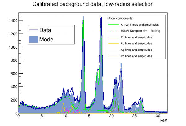 |
| Assumes Compton component has same resolution as the lines | Assumes Compton component has resolution twice as bad as the lines |
Details on the above fits:
- Each component is separately fit, but within a component published branching fractions are used
- The peaks are gaussians using the resolution function, with low-energy tails added. The tails are adjusted so that 37% of the peak is in the tail, and the tail is an exponential with length 5% of the peak energy (i.e. I assume a linear dependence with energy)
- The 60keV Compton component was originally scaled based on simulation results and published branching fractions with respect to the 14keV line. However to fit the curve the amplitude had to be increased by a factor of 1.6. This may suggest that the attenuation of 14keV gammas c/w 60keV gammas is stronger with the actual source and collimator than with the simulation.
- The model does not reproduce the 8.5keV Au line very well, because it sits right on the steeply falling edge of the Compton curve. The Compton simulation was smeared with the standard calibration (left plot), but if you assume the resolution is 2× worse (right plot) it does a better job with this peak. The Compton events are spread over a larger region of the detector so maybe the resolution is worse.
TODO
- Redo spectrum with Nick's new cut recommendations, compare
- resolution: check cearly vs clate vs corrected vs 2template vs tail cut
Resolution versus Energy
Fits were performed on the visible lines to estimate their resolutions. For the 14keV line and the four lines below it, I used a gaussian + flat background. For the higher peaks, each overlaps significantly with a neighboring peak, so I used double- or triple-gaussians + flat background.
A fit of resolution versus energy was done. I added a zero-energy resolution point of 10±5 keV, and the fit was the sum of a constant term and a sqrt(energy) term. I rejected several lines that were anomalously wide: the 12keV gold line, which is widened by a nearby americium line, and the 17keV, 21keV, and 25keV lines, all of which are the left line of a double/triple line, and all of which seem to have extra tails trailing off to the left. I don't know why those tails are there - they seem more prominent in higher energy lines, with very little tail seen in the 14 keV line. Perhaps they are related to saturation. The rightmost lines in the double/triple lines show a sharp right edge and are thus relatively narrow according to the fits.
$res = \sqrt{res0^2 + f \times \epsilon \times E}$, with constant ε = 3.8 eV.
| Figure 5.1 | |
|---|---|
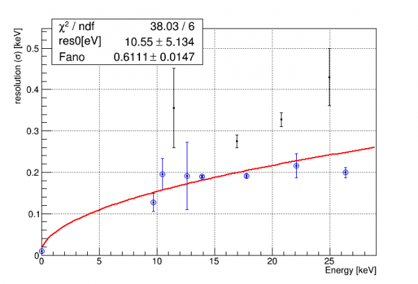 |  |
The highest line seems too narrow and does not fit the curve well - it's conceivable that maybe it is distorted (“squished”) by saturation effects. If we leave it out we get the following:
| Figure 5.2 | |
|---|---|
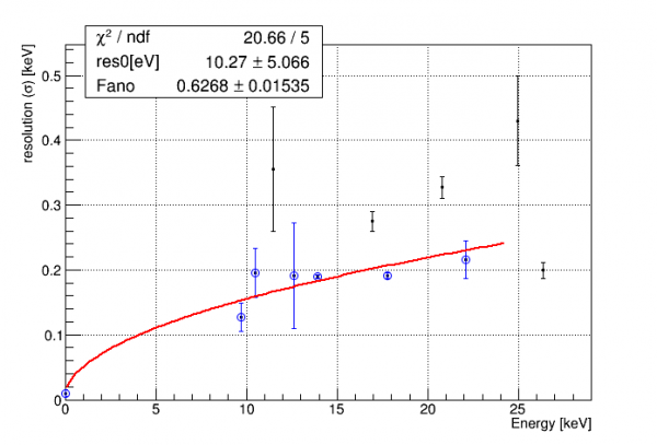 | 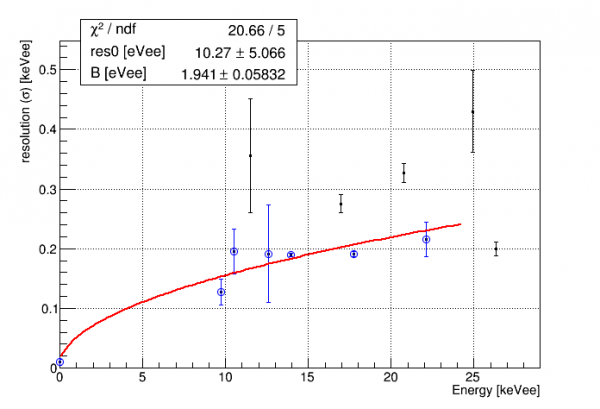 |
| This should be considered the best resolution function. | This is the same fit, but with a different parameter definition, see below. |
For the purposes of fitting NR events, Nick redefined the parameters of this resolution function. I originally used an effective Fano factor (left plot in Fig 5.2). Since we expect a different Fano factor for NR events, Nick separated out the accepted silicon Fano factor (which assumes ER events) from any other root-E dependency in the resolution. This new, separated factor is assumed to be some detector effect that holds for ER and NR alike. The new fit function is
$res = \sqrt{res0^2 + (B+f \epsilon) \times E}$, with constant ε = 3.8 eV and constant f=0.1161. Parameters res0 and B are both in energy units.
If we want an idea of the systematic error we can try a different fit with more terms. I tried the following:
$res = \sqrt{res0^2 + f \epsilon E + E^2/eprop}$; as above but with an energy-proportional term, with dimensionless parameter “eprop”.
When I try fitting to the same curve as before, the energy proportional term is heavily suppressed, and the 0-energy resolution and Fano parameters come out exactly the same as in the 2-parameter fit.
As an alternative we can remove the two highest-energy points, and fit both the original 2-parameter function and the new 3-parameter function to the lowest-energy points:
| Figure 5.3 | |
|---|---|
 |  |
| These are alternative resolution fits, mostly to give an idea of the systematic uncertainty in the parameters. | |
Note in the above that the Fano factor is a lot smaller in the 3-parameter fit, but the errors are very large - large enough that it is in fact consistent with the previous value. In the 2-parameter fit the removal of the higher-energy lines has a small effect.
Compton Step search in -125V Na-22 data
In Run 68 we took a lot of data with the Na-22 source (1.2 MeV gamma) in order to produce a Compton spectrum. At low energies there should be steps in the spectrum corresponding to silicon energy levels, which could serve as calibration features. There should be a step at 1.839 keV (12:14 ratio of event rates below:above this value) and a step at 0.099 keV (4:12 ratio of event rates below:above this value). Unlike with features from the Am source these events should be uniformly distributed throughout the detector.
Early attempts
The plots below represent early attempts to see the Compton step, before all of the details of the Am spectrum had been worked out and before the quality cuts had been fully developed.
| Figure 6.1 | |
|---|---|
 | 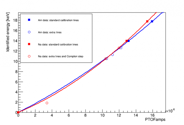 |
| This uses the 2-template OF amplitude with baseline correction and a fiducial cut applied. Green line is where the 1.839 keV step should be according to the Am calibration. | Above indicates that the step identified does not agree with the Am calibration |
Updated attempts
Since the early attempts above two things have happened. First, a fuller understanding of the spectrum from the Am source, including all the fluorescence lines, has given further confidence to the quadratic fit to the 14 and 18 keV lines, since it seems to fit well to lines down to 8 keV. It's still not certain how well the calibration works for events not near the central axis, but there are indications that the channel balancing works so the default assumption should be that the calibration is good for higher-radius events as well. Second, Nick has tuned the quality cuts to remove pileup and tails and so on, with the intention of minimizing energy bias in the cut efficiency.
The analysis in this section uses Nick's standard cuts and corrections as of 2019 March 10 (as of this time the cut to remove clustered low-energy events is not finished). The standard calibration based on pT OF and the Am lines is used.
1.839 keV step in Na data
The plot below shows the expected step shape overlain on the low-energy Na spectrum.
| Figure 6.2 |
|---|
 |
| The only free parameter in the fit is the overall amplitude. The step position and height are fixed to their expected values. The step width was chosen arbitrarily and fixed. |
There's little convincing evidence of the 1.8 keV step in the plot above. There may be some hint of it at a too-low energy and rather poor resolution. The overall spectrum is improved compared to the earlier analysis because it is reasonably flat as expected - the previous analysis probably had energy-dependent cut efficiencies.
The plot below is also the Na spectrum but selecting only events with high pF partition, to test the idea that the calibration may work better for low-radius events.
| Figure 6.3 |
|---|
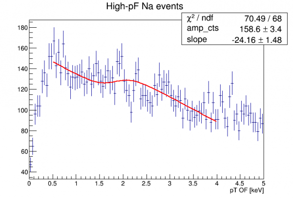 |
| The free parameters in the fit are the overall amplitude and an overall slope. The step position and height are fixed to their expected values. The step width was chosen arbitrarily and fixed. |
The low-radius Na spectrum above has an overall downward slope. This could be because this is mostly Am events, and therefore mostly the 60 keV Compton spectrum, which would have a noticeable downward slope in this energy range. It could also be because the high-F and low-F distributions flare out at low energies as the relative partition resolution gets worse, so that at lower energies there are more low-F events leaking in.
There's better evidence for the 1.8 keV step above, but the stats are pretty low and the extra arbitrary slope parameter means it's easier to make a fit work even if it isn't physical.
0.1 keV step in Na data
We can also look for the lower step near 0.1 keV. The stats are lower, but the step height is greater (a 3-to-1 ratio) so there's a chance to see it.
But this energy region is polluted by the low-energy clustered junk events discovered by Nick. One of the ways to remove these is based on the pA partition, because these junk events have anomalously high energy fractions in the outer-ring channel pA.
| Figure 6.4 |
|---|
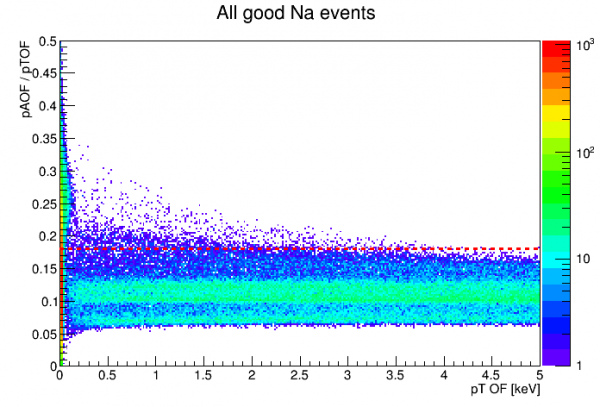 |
| The red dashed line is a threshold for a pA-partition cut. |
The pA-partition cut pictured above serves to remove most of the junk events, and also in principle serves as a fiducial cut to remove high-radius events.
| Figure 6.5 |
|---|
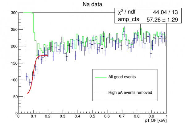 |
| The only free parameter in the fit is the overall amplitude. The step position and height are fixed to their expected values. The step width was chosen arbitrarily and fixed. |
The plot above shows a pretty good hint of the lower Compton step. To evaluate this fully we should wait for the trigger efficiency analysis - it's possible the step seen is actually a trigger artifact, or partially so.
0.1 keV step in background data
I also looked in background data. There is less than half as much background data as there is Na data. As it turned out the statistics are too poor to attempt a fit of the 1.8 keV step. However there is some indication that the lower step is seen as in the Na data.
| Figure 6.6 |
|---|
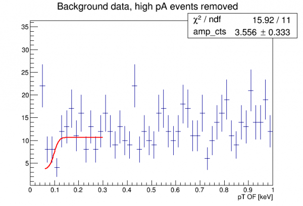 |
| The only free parameter in the fit is the overall amplitude. The step position and height are fixed to their expected values. The step width was chosen arbitrarily and fixed. |
Absolute phonon calibration
The purpose of this section is to try to further understand our default energy calibration. This was inspired by the Migdal Effect analysis, which suggests a Migdal peak which may correspond to an observed feature in our PuBe spectrum, but only if our calibration is pretty far off at low energies. The Migdal peak should be at 110 eV, which is only 65% of where the feature appears according to the calibration: 170 eV.
The default calibration of PTOFamps is based on the two Am lines at 14 and 18 keV. It is a quadratic fit constrained to (0,0). It appears to be a good fit to the four visible lower lines, down to about 10 keV. The question remains whether this is reliable all the way down to around 0.1 keV. (Probably the best indication that it should be close to correct down to energies so low is the observation of the 10keV, 1keV, and 0.1keV lines in the GeHV detector, with no clear indication that the 0.1 keV line was very far from where it was expected.)
The OF quantity has complicated behavior. An absolute calibration based on pulse integrals should be simpler. If calculated correctly and if regimes of true saturation are avoided it should be linear with energy (since phonon collection efficiency is presumably a constant).
Non-linearity of default calibration
There are a few possible things that could contribute to the nonlinearity of PTOF calibration:
- the fundamental non-linearity of the TES response
- the change in pulse shape at higher energy
- true saturation effects (which seem to be very small below 20 keV)
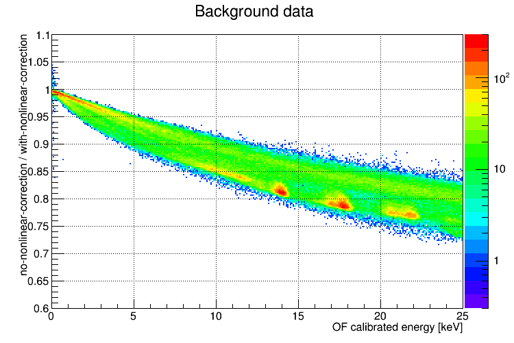
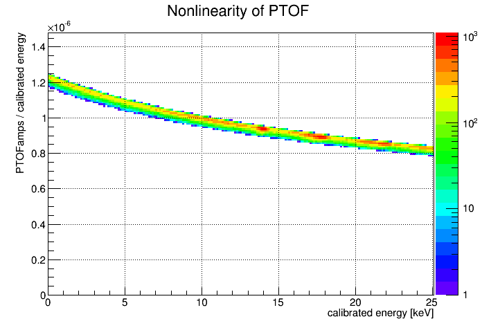 | This plot shows the ratio of raw PTOF amplitude to energy as a function of energy. The energy used is the standard OF calibration, so this simply another way of showing the calibration curve. (The reason there is some thickness to the curve is that no baseline-correction has been applied to the raw OF amplitude.) Amplitudes from the OF algorithm fall off with increasing energy. The nonlinearity can be quantified as follows: amplitude/energy is 4.8% smaller at 17.75 keV than at 13.9 keV. |
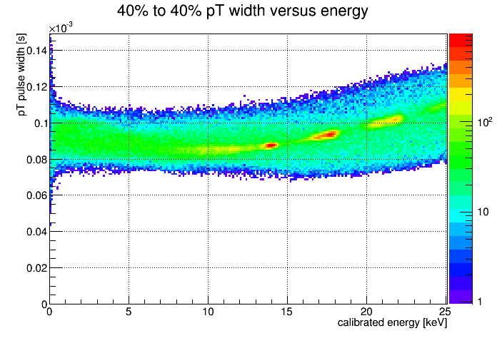 | The PTOF pulse shape varies with energy as seen in this plot of pulse width versus energy. This is one reason why the OF amplitude based on a single template is not linear with energy. The width at 17.75 keV is about 7% larger than at 13.9 keV. |
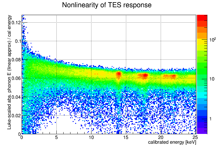 | This plot uses the absolute phonon calibration based on IbIs information and pulse integrals. Here the correction for nonlinear TES circuit response is not applied. The linear approximation of absolute phonon energy is scaled to (OF-calibrated) energy and plotted versus energy. The amplitude/energy is 2.0% smaller at 17.75 keV than at 13.9 keV. So this accounts for only some of the nonlinearity of PTOF. |
Linearity of absolute phonon calculation
In this section I apply the fully-calculated absolute phonon energy, including a correction for nonlinear TES response. This correction gets stronger with pulse height above baseline, so the correction is larger at higher energies and it is also larger for peakier pulses. The correction is calculated from pulse shape using walk algorithm timing quantities.
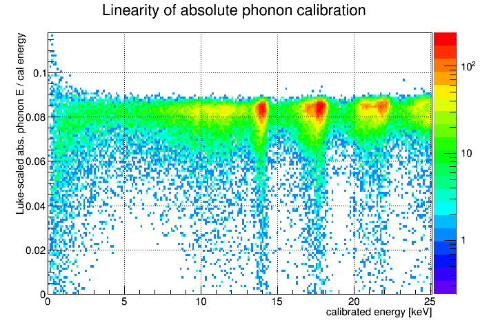 | Using the standard OF-calibrated energy as a reference, this plot shows the linearity of the absolute phonon energy calculation over a wide range of energies. Or, if we trust that the absolute phonon calibration is correct and that the phonon collection efficiency is constant with energy, then the flatness of this plot suggests the OF-calibration is correct over a wide range. The absorbed phonon energy has been scaled by the Luke gain, assuming 125 V bias. In this way the value on the vertical axis can be read as phonon collection efficiency for the readout side of this SiHV detector. |
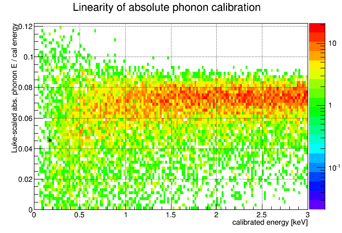 | Same plot as previous but zoomed in to low energies. Here there is a hint of a falloff at low energies. This could be interpreted as a possible bias in the OF-calibration that overestimates energies below 1 keV. An asterisk has been added to indicate where we'd see the Migdal peak, if the OF calibration were overestimating its energy by a factor of 170/110. |
Is there a conceivable reason why the OF amplitude would be biased to overestimate energies significantly only at very low amplitudes? To investigate I looked at events around 0.5 keV. In Na-22 data, which is much higher-rate data, the effect was perhaps stronger, with a significant number of events actually showing negative absolute absorbed phonon energy. Looking at traces it was clear why - many traces are on downward-sloping baselines. The integral algorithm uses the prepulse to set the baseline and integrates over the full trace, including a long time after the pulse, so a downward slope will result in a too-low integral, not indicative of the pulse amplitude. The effect will of course be relatively stronger at small energies.
Nick developed a simple method to correct pulse integral quantities in the case of a downward-sloped baseline. I applied a similar correction to the absolute phonon calibration.
Linearity of absolute phonon calibration with a correction for sloped baselines


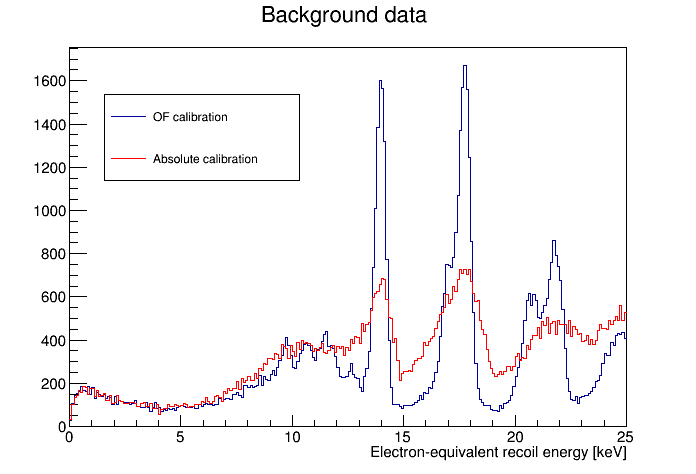
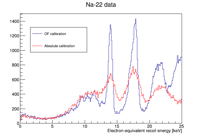
Further look at OF calibration linearity checked against absolute calibration
 |  |
 |  |
 | |
 | |
 |  |
 |
|
 |  |