Table of Contents
Activation with PuBe Source
On Dec 6th we began activating the detector with the PuBe source in it's transport drum, behind the thick lead wall. The purpose of this activation was to measure the thermal neutron flux at the detector by observing the growth of the 10keV activation peak with time.
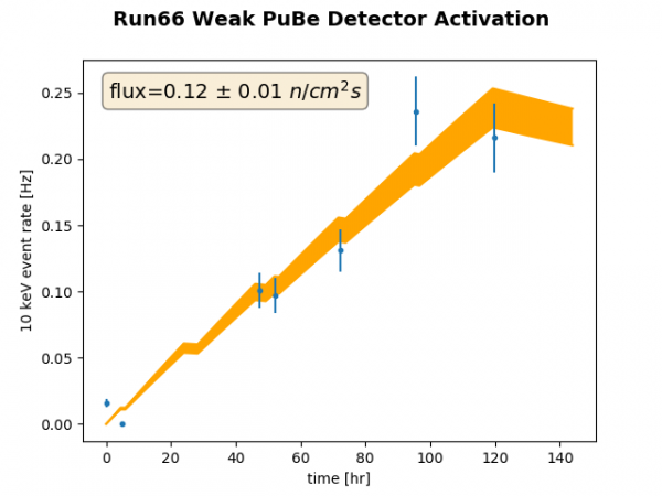 | 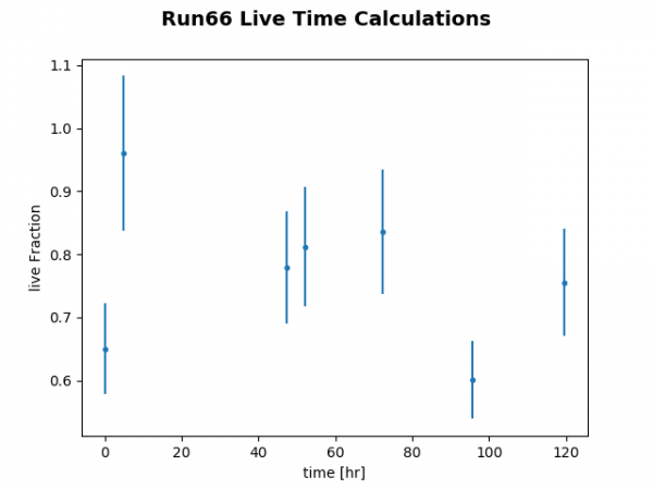 |
| Weak PuBe activation. Blue points are measured 10keV event rates calculated from fits to the PT integral peak and live time estimates. Orange band is the fitted activation model with uncertainty in activation rate. The two outliers (first and second-to-last data points) both have low livetime fractions (right). |
|
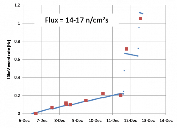
On Dec 11 and 12 we performed two 2-hour strong activations with the PuBe source lowered into the corner of the cryostat lead/poly shield. The plot below shows the 10 keV rate during both the weak and strong activations and an approximate fit.
| Run 66 Weak and Strong PuBe Activations |
|---|
 |
More thorough estimate of PuBe activation rates
To estimate the rate of 10keV events from activation of Ge-70, we have to account for the read efficiency of the DAQ. We now know that the data we have from the activation periods had reduced read efficiency due to the fact that long risetimes can cause the DCRC to retrigger an event, and the original version of the MIDAS trigger front-end used a pileup rejection that would throw out both triggers. Since then the front-end has been modified to keep the first trigger in a “pileup” (or retrigger).
The read efficiency can be expected to be energy- and position- dependent since it depends on pulse shape. This needs to be taken into account when estimating the read efficiency for events in the 10keV peak. This is one reason to redo the activation rate calculation. Another reason is to more thoroughly account for error in the measurement. This is motivated by the fact that simulations do not agree well with the observed activation rates, and the ratio between them, for the two PuBe source positions. The simulated ratio between the strong and weak fluxes is around 400, significantly higher than the observed ratio of around 100.
To calculate the read efficiency we get the rate (in Hz) of pulses in randoms and compare to the rate (in Hz) of pulses in triggered data. This requires a criterion for identifying events with pulses in either random or triggered data, and events passing this hit criterion should be high enough in amplitude that they should normally produce a trigger. We use a threshold P$WKmax, the peak height of the triggering phonon channel as determined by the walk algorithm.
| Figure 1 |
|---|
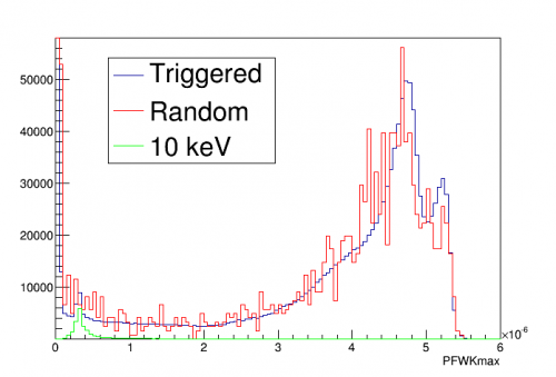 |
| Comparison of spectra in randoms (scaled up) and triggered data This includes all data taken during the weak and strong activations Also shown is a spectrum specifically of events around 10keV |
| Figure 2 |
|---|
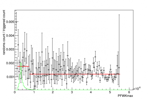 |
| Ratio of randoms spectrum to triggered spectrum The 10keV spectrum is overlaid in green, and fits of two regions are shown in red Events around 10 keV have a higher randoms/triggered ratio (thus lower read efficiency) |
Figures 1 and 2 above show that the shape of the triggered spectrum is a rough match to the randoms, but there seem to be some systematic differences with energy, which would mean the read efficiency is energy-dependent.
| Figure 3 | |
|---|---|
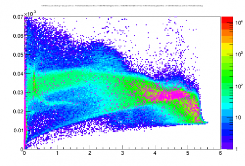 | 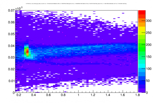 |
| Risetime of the triggering channel pF versus peak height, in triggered data (color map) and randoms (magenta dots) | |
From what is understood of the loss of read efficiency from DCRC retriggering, the risetime of the triggering pulse should be important - long risetimes produce retriggers. Figure 3 above shows that the risetimes tend to be larger for lower energy events, and in particular there's a hint that the 10keV peak events have longer risetimes than other low-energy events. This could have a sensible physical reason: 10keV peak events are bulk, but most background at such low energies will be near-surface gammas, and near-surface events could have quicker risetimes on average. Thus it's possible that 10keV peak events have worse read efficiency than most events.
For estimating the read efficiency of 10keV events this presents a problem. There seems to be an energy dependence so we need to measure the efficiency at amplitudes near the 10keV region. If we use a global read efficiency for all the data there may be enough statistics - but unfortunately there seems to be a time dependence in the overall read efficiency (perhaps correlated to increasing event rate). So the main strategy I employed was to calculate separate high-amplitude efficiencies per series, but use a global correction based on all the data to scale this for the 10keV region.
To calculate the observed 10keV rate in triggered data I simply count the events in a wide window around the peak (4-14 keV) and subtract the counts in an equal-sized window above the peak (15-25 keV).
| Figure 4 |
|---|
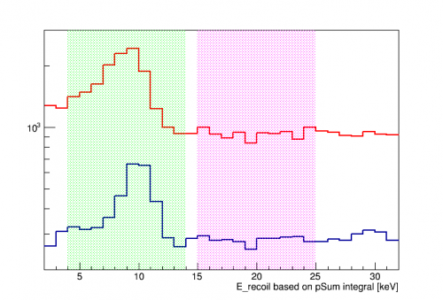 |
| Selection windows for counting events in 10keV peak and subtracting background Red = data after strong activation Blue = data towards end of weak activation |
| Figure 5 |
|---|
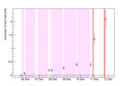 |
| Calculated 10 keV event rates at different times Shaded regions show periods of weak (magenta) and strong (red) activations |
Figure 5 above shows the calculated 10 keV rates using the method above: count events in the peak region, subtract background, and adjust based on read efficiency, both a high-amplitude efficiency per series and a fixed correction to the 10 keV region. Also shown are the periods during which the source was present for activation in its two positions.
The information in Figure 5 can be used to estimate the activation rate from the PuBe source in its two positions (weak and strong activations). I define activation rate in Hz as the number of Ge-70 nuclei in the crystal activated per second. This is the rate at which Ge-71 is generated.
Given a decay rate τ (halflife/ln(2)) and activation rate A between times t1 and t2, the change in decay rate R2 versus R1 is
$$R_2 = A + (R_1-A)e^{-(t_2-t_1)/{\tau}}$$
Note that if the duration is much greater than τ the decay rate R approaches an equilibrium value equal to activation rate A.
Suppose we have a series of activation periods: A1 between t0 and t1, A2 between t1 and t2, etc. Also assume that before t0 there is an ambient activation A0 - then we know that at t0, R=A0. At any later time t the decay rate is
$$R(t) = A_{m+1} + \sum_{i=0}^m(A_i-A_{i+1})e^{-(t-t_i)/{\tau}} $$
where “m” denotes the index of the end time of the most recent activation period.
For the model I assume three activation rates: A_ambient, when there is no source present, and A_weak and A_strong. During the weak activation periods the rate is A_ambient+A_weak and during the strong activation periods it's A_ambient plus A_strong. The 10 keV rate is not equal to the decay rate R, it's equal to fR, where f is the branching fraction for K-shell electron captures, taken to be f=0.87. Fitting the data to this model yields the following:
| Figure 6 |
|---|
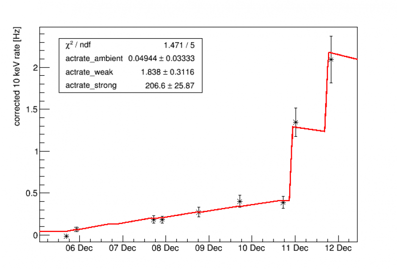 |
| Activation rates fit to 10 keV rate data |
If we want to make the connection between the activation rate and the neutron flux, we need the number of Ge-70 targets in the crystal and the effective neutron capture cross-section. Using the abundance of Ge-70 in natural Ge (20.5%) and the dimensions of the detector (radius 5 cm, thickness 3.3 cm) I calculate 2.345e24 Ge-70 nuclei. The capture cross-section is highest for the lowest-energy neutrons, so if we take a capture cross-section for thermal neutrons we can estimate an approximate thermal neutron flux. Sources differ on this, e.g. 3 bn from NIST and 5 bn from JENDL. In general we can say
flux [/cm^2/s] = A [Hz] / (2.345 × σ [bn])
| A [Hz] | error | Flux (3bn) [/cm2/s] | error | Flux (5bn) [/cm2/s] | error | |
|---|---|---|---|---|---|---|
| ambient | 0.049 | 0.033 | 0.0070 | 0.0047 | 0.0042 | 0.0028 |
| weak | 1.84 | 0.31 | 0.261 | 0.044 | 0.157 | 0.027 |
| strong | 207 | 26 | 29.4 | 3.7 | 17.6 | 2.2 |
We can add data from late in the run, after the read efficiency problem was solved by changing the MIDAS trigger front-end. The read efficiency still must be taken into account: it's a little above 90% not 100%. I'm not sure why there is still some loss, or whether there is something that I'm neglecting in the calculation. But there is no reason to assume it is pulse-shape dependent.
| Figure 7 |
|---|
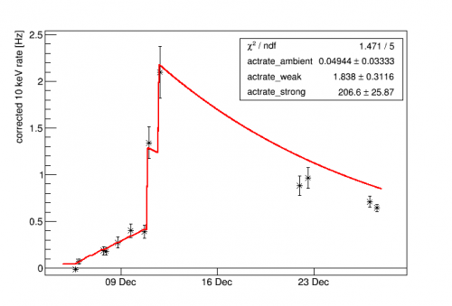 |
| Activation fit with late data added. The fit is only to the earlier data, as in Figure 6. |
As can be seen in Figure 7 the 10 keV rate in late data falls below the fit curve. This suggests that the early data has been over-corrected - the estimate of the read efficiency (high-amplitude corrected for the 10 keV range) for the early data seems to be too low.
As stated above we don't expect an amplitude dependence in the read efficiency for this later data. However empirically there seems to be a similar difference between low amplitudes and higher ones:
| Figure 8 |
|---|
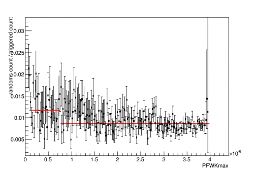 |
| Ratio of randoms spectrum to triggered spectrum in late data This is after the event loss due to DCRC retriggering was rectified. |
I'm not sure why there seems to still be this discrepancy. Perhaps there are systematic differences between how the walk algorithm finds a maximum in randoms, where the pulse can be found at any time, and in triggered events, where it is always in the same place. At any rate if we apply a similar correction to account for high-amplitude versus low-amplitude efficiency, the later data points fit the earlier ones well:
| Figure 9 |
|---|
 |
| Activation fit with late data added, this time with an efficiency correction for low-versus-high amplitude. The fit is only to the earlier data, as in Figure 6. |
Update: selection criteria for randoms when calculating the event rate
As mentioned there should be no energy dependence in the read efficiency for the later data, after the trigger front-end problem was remedied. The fact that there appears to be one (Figure 8) suggests that there is a problem in the calculation.
Originally to select randoms with pulses, a threshold on P$WKmax (the maximum of the trace above baseline, for the triggering channel) and no other cuts. A closer look reveals problems with this. One is that the algorithm will fail if the pulse appears too early in the trace, because the baseline is calculated from the first few hundred samples, so if the peak is within that window the baseline will be overestimated. So I tried applying a restriction to the peak time, P$WKr100.
Before applying the peak time restriction, the read efficiency around 10 keV relative to higher energies for late data was 0.74 +/- 0.04. After applying the peak time restriction there is a small improvement: 0.80 +/- 0.12. But there is still a clear energy dependence.
Another problem is dealing with pulses that appear on tails of previous large events. I looked at randoms in the 10keV range, and the 12th such random appeared on a tail:
| Figure 10 |
|---|
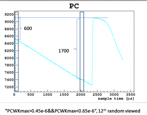 |
| Example pulse for which the walk algorithm will produce a higher amplitude for random versus triggered |
In the pulse above the walk algorithm produces a much smaller amplitude than it would have if it were a triggered event, because if it were triggered the baseline window would come later, at a lower point on the tail. Hence we can expect that the amplitude spectrum in randoms will be shifted to lower amplitudes relative to the triggered spectrum.
To deal with this I applied a second selection criterion on randoms: a tails cut. The basis of the cut was to remove events whose baselines were higher than the average value. The cut was tuned to a 98% efficiency when applied to randoms (after the peak time selection). When this selection is applied to randoms and triggered data the ratio of the randoms and triggered spectra is flatter. The read efficiency around 10 keV relative to higher energies becomes 0.95 +/- 0.06. Thus within error there is no energy dependence to the read efficiency, as should be the case.
I then took a second look at data taken during the activation, before the trigger algorithm had been fixed. The read efficiency around 10 keV relative to higher energies turned out to be 86%, in contrast to the 65% seen before I tried applying randoms selection criteria. So the 86% is probably closer to the true energy dependence of the read efficiency caused by the retriggering/trigger algorithm problem.
Below are some results of activation rate estimates after applying these new selection criteria to calculate true event rates from randoms and read rates from triggered data.
| Figure 11 | ||
|---|---|---|
| no energy-dependent correction to late data | with energy-dependent correction to late data | |
| fit only early data | 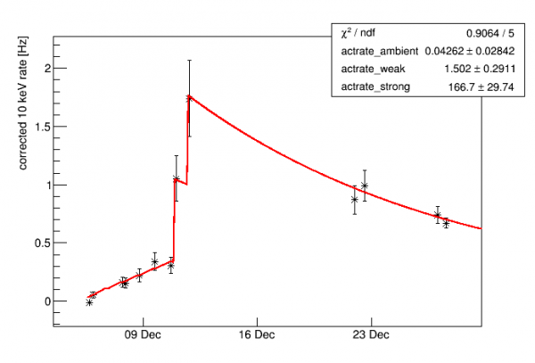 | |
| remove early data after strong calibration |  |  |
| fit all data |  |  |
Figure 11 above shows a few options for fitting the activation rates. First there's a fit to only the early data, and here we see that the curve fits the late data points too. The second row shows the results if we remove the two early data points that occur after the strong activations. This is nearly the same as the third row, which fits all the data (the errors on the rates in later data are much smaller and drive the fit). On the left is the case where we use high amplitude events to calculate the read efficiency of the late data, which turns out to be on average 97 +/- 5 %. On the right is when we apply an empirical correction to the read efficiency for the 10keV region, reducing the efficiency by another 5%.
The final result is the bottom row, either with energy-corrected efficiency in the late data or without. (The two different values for the strong activation differ by about 1 sigma.) My inclination is to include the correction. This makes it internally consistent with what is done for the earlier data, and may account for some small remaining systematic in the comparison between randoms and triggered data. So the final result then is the rates in the bottom right of Figure 11.
The new method produces higher efficiency estimates, so this correspondingly produces lower fit values (about 80% as high) for the activation rates as compared to Figure 6. The ratio between the strong and weak activation rates is nearly the same.
As stated previously, the activation rate can be converted to a neutron flux if we assume an effective capture cross-section with
flux [/cm^2/s] = A [Hz] / (2.345 × σ [bn])
The cross-section estimates vary between 3 and 5 barns. Below I use 3.71 barns to quote a flux estimate (this is a value that I think Anthony was using at some point).
| A [Hz] | error | Flux (3.71bn) [/cm2/s] | error | |
|---|---|---|---|---|
| weak | 1.49 | 0.29 | 0.171 | 0.033 |
| strong | 172 | 12 | 19.8 | 1.4 |
Appendix: PuBe source dimensions
The PuBe source is in a steel can which fits into a tube that extends down into a paraffin-filled barrel. Inside the can itself is a solid object, either the source or a casing that holds the source, a few cm in size.
| Barrel outer diameter | 41.5 | cm |
|---|---|---|
| Barrel height | 54.5 | cm |
| Depth from top of barrel to top of paraffin | 9-10 | cm |
| Depth from top of barrel to bottom of tube | 28.5 | cm |
| Outer Diameter of steel can | 4.5 | cm |
| Height of steel can | 11 | cm |
| Height of PuBe source in steel can | 5.5 | cm |
| Elevation of bottom of source from bottom of barrel | 26 | cm |
| Elevation of top of source from bottom of barrel | 31.5 | cm |
Other details are given in the PuBe Source information page
Howitzer
The howitzer containment for the source is cylindrical with the following dimensions:
| Diameter | 30 | in |
|---|---|---|
| Height of main body | 31 | in |
| Full height including wheels and c-rings on top | 38 | in |
| Weight, including locks and inserts (but not source) | 864.5 | lbs |
| Weight, with locks and inserts removed | 857.0 | lbs |
The source can on its lucite rod can be lowered into the top of the howitzer. A lid can be placed over the rod and padlocked.
The howitzer has three ports along the diameter halfway up which allow samples to be placed near the source in the center for activation. There also seem to be three vertical sample ports at the top for the same purpose.
It is not known what the howitzer is made of. Presumably it is mostly neutron moderating material. The visible surfaces seem to be painted steel or another metal. As far as can be seen there is no dedicated gamma shielding, e.g. lead.
The dimensions above imply an average density around 1.1 g/cm^3. HDPE has a density of 0.94 g/cm^3.