Table of Contents
Run 58 Summary
USD1 description and preparation
The detector USD1 is a Ge crystal from USD fabricated at TAMU with a 4-Q mask.
The detector arrived at UMN sans housing in a shipping container. On 2016 March 16 we dismounted G101b from its housing and shipped it to TAMU. This is a 2-DIB housing for a 100mm detector. The former G101b housing was used to mount USD1 on 2016 April 27. The detector was wirebonded on 2016 May 2nd, 3rd, and 23rd.
The detector is mounted such that the charge side faces up (away from tower). If we'd like the Am sources to face the charge side, the source holder must be mounted 1 position above (further from the tower than) the detector.
The wirebonding is done as follows:
| USD1 pinout map | ||||
|---|---|---|---|---|
| q1 | q3 | q2 | q4 | g |
| DIB1qO | DIB1qI | DIB2qO | DIB2qI | DIB1pin7 |
| Charge channels are numbered outer-to-inner | ||||
| A “1” is scratched onto housing above DIB1 (a little hard to see) | ||||
| DIB1 is the DIB nearest to the housing serial number | ||||
q1, q2, q3, q4 refer to the four charge channels numbered outer to inner, so q4 is the innermost and q1 is the outer ring.
g refers to the ground connections, wired to QET Return line D on DIB1. (Originally QET return lines B and C were used, but it was changed to D on May 23rd. This will allow us to use the HV board with DIB1 attached to HV1.)
The ground side of the detector seems to be a uniform Al electrode rather than a grid - previous 4-Q devices had grids on the ground side. This may impact the ability to neutralize the detector with LEDs.
There were only two working LEDs, one on each DIB, according to the electrical checkout. Previous checkouts for G101b (from 2011 to 2014) indicated three working LEDs. One LED had apparently been open since the detector was shipped to UMN. It seems one of the remaining LED wirebonds was broken during mounting or wirebonding.
A visual inspection was done with the lids removed to identify which LEDs are on which sides, and to see if the wirebonds from the LED to the neighboring DIB pad were visible:
| LED | Side | Checkout status | Bond visible | Previous checkout status |
|---|---|---|---|---|
| DIB1 LED1 | ground | bad | no | good |
| DIB1 LED2 | charge | good | yes | good |
| DIB2 LED1 | ground | good | yes | good |
| DIB2 LED2 | charge | bad | no | bad |
| note that the DIB numbering is apparently opposite now from the previous case | ||||
On May 23rd the two bad LEDs were wirebonded. Now all four LEDs pass the electrical checkout.
Readout scheme
iZIP-style biasing with the DCRCs
If we plug two DCRCs directly to the two DIBs, we can set each charge channel on both DIBs to the same voltage, and the ground side will remain grounded. In this way we can bias in a range -12 to +12 V.
Biasing with the HV board
To use the HV board we would want DIB1 to be connected to HV input 1, because that HV input will read out the charge channels and apply HV to pD. DIB2 would connect directly to a DCRC. Then the HV board would allow us to bias from -100 V to 100 V or more, this time with the “ground” side biased and the charge side left at ground potential. (We could also do symmetric biasing in this scheme by using the DCRC bias to apply voltage to the charge side and the HV board to apply opposite bias to the ground side.)
Electrical problems
- q3 connection: The q3 (DIB1qI) connection seemed to go bad between the 300K and 77K electrical checkouts. The qBias-to-QET-return check which should have been 25 nS only read 13 nS. Later this channel was seen to only rarely show large pulses. Possibly a wirebond came loose. This connection seemed OK again at 300 K. Wirebonds were examined and no issues seen.
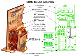
- Short to chassis: The pD Feedback loop is shorted to chassis on both DIB1 and DIB2. Specifically the Coil line seems to be shorted in both cases, since its resistance to chassis is smaller than the Return to chassis. At 100 K while cooling the DIB1/DIB2 coil-to-chassis resistances were 7/1 kΩ. Since DIB1 pD is connected to the ground side of the detector, this short led to high leakage current when we tried to use the HV board - we had to use a switchboard to disconnect the Feedback loop in order to run the HV board. When uninstalling it was seen that these shorts were where the SQUET flyover cable comes into contact with the stripline plug chassis.
The short to chassis at the SQUET was similar to the one from Run 57. In that case the short was at QET A. Examining diagrams of the SQUET it was found that the outer flyover cable, the one that can come into contact with the plug chassis, holds the four twisted pairs for pA and pD. The QET-A-to-ebox pair is on the far left, and the Feedback-D pair is on the far right, if you are holding the SQUET upright on its fridge mount and looking at the SQUID card side. So not surprisingly it seems that the shorts have shown up in the twisted pairs on the far ends of the outer flyover cable.
For future runs we are trying to prevent such shorts with a kapton tape reinforcement in the appropriate place on the outer flyover cable.
Measurements
Breakdown voltage
As we increased the bias on the crystal we looked for signs of breakdown by observing the charge channel readouts and looking for distortions. Using the DCRC only (which applies bias to the top (charge) side of the crystal and grounds the bottom side) we saw no breakdown up to voltages of +13 V and -13 V. At all voltages the channels showed normal pulses with no distortions or unusual noise states.
Using the HV board (after dealing with the chassis short mentioned above) we were able to apply higher voltages. Using the HV board alone applies a bias to the bottom of the detector, with the top left grounded. Using the HV board and the DCRC together, with the DCRC applying the opposite bias, allows for symmetric biasing on both sides of the detector.
The HV bias was calculated from the applied voltage and the measured leakage current by calculating the voltage drop across the 400 MΩ bias resistor. Leakage current varied from 1 to 5 nA normally, but was typically higher (up to 10 nA) and unstable when breakdown was occurring. This might suggest that measurable current (up to 5 nA) was leaking through the detector. At the highest crystal biases tested (15 V) this would dissipate 75 nW at the base, which would not cause a noticeably change in base temperature.
Breakdown symptoms were seen at around +16.5 V and -15 V (where + indicates that the top was biased higher than the bottom). These were the results of one-sided biasing. With symmetric biasing the positive breakdown was similar but the negative breakdown was about -16.5 V.
When applying biases to the four charge electrodes it was seen that when there was a bias difference between two channels, breakdown symptoms were seen even at only a few volts. This is not surprising due to the cross-channel resistances.
Charge collection efficiency
| Using the high-energy blob to determine scaling factors btwn spectra |
|---|
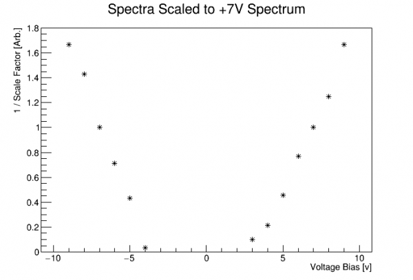 |
Ideally, we'd use peak locations to estimate relative charge collection efficiencies - but no peaks are visible. The large change in trigger rate suggests that the low-energy range of the spectrum may not be comparable across voltage biases. But the muon blob is a high-energy feature that, if present, might be used to safely compare calibrations from different bias voltages.
update
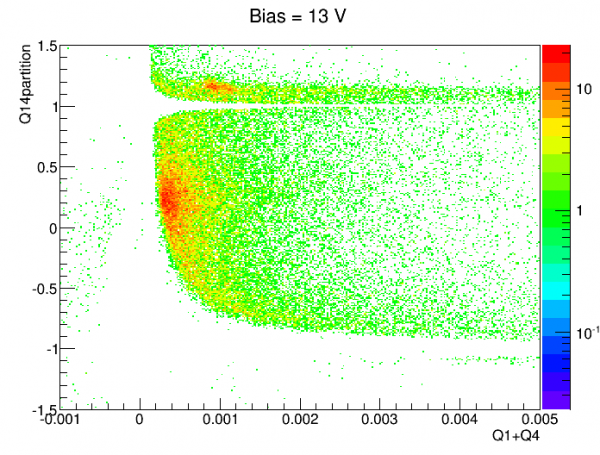
After tinkering with charge partition plots, I finally found a way to see the 60keV peak in Q1 (the outermost channel). I defined partition quantities between Q1 and Q4 (outermost and innermost) and Q1 versus Q2 (outermost and second outermost):
z->SetAlias("q14part","(q1-q4)/(q1+q4)")
z->SetAlias("q12part","(q1-q2)/(q1+q2)")
|  |
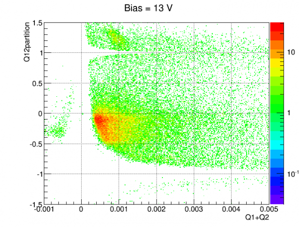 |
In the plot on the left above the band near q14partition=1 can be interpreted as Q1-dominant events, with little to no signal in Q4. Note the red patch near Q1+Q4=0.001 - this seems to be a 60keV peak in Q1. It can also be seen in the plot on the right. I define cuts:
TCut c1n4 = "q14part>0.7"
TCut c1n2 = "q12part>0.7"
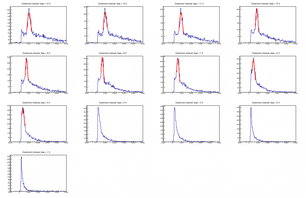
to select events in which Q1 is dominant over Q4. With this selection I created Q1 spectra at each bias:
| Q1 spectra with partition cut, positive biases |
|---|
 |
| Q1 spectra with partition cut, negative biases |
|---|
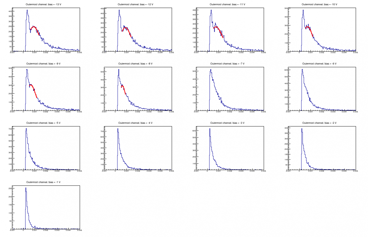 |
Where peaks are visible I attempted to fit them with gaussians. The peak hard to distinguish at positive biases less than 5 V. At negative biases the peak is broader. It makes sense that positive biases produce cleaner peaks because these are hole-events rather than electron events, and holes travel straight along field lines unlike electrons.
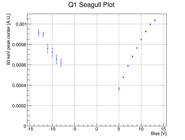
Below is an attempt at a seagull plot based on the peak fits. It seems to be a pretty good match to the plot generated using the high-energy spectrum. Combining these plots could produce a more complete one since each includes data points the other lacks.
Neutralization hold time
Comparisons with other detectors
In Run 11 the first 100mm 4-Q device was studied.
Event Rate
To troubleshoot why no peaks are seen, one thing to check is the raw event rate. Is the rate what would be expected from four Am sources and with no lead+poly shield erected around the fridge?
For two reasons the trigger rate can't be used to estimate the event rate. First we know the trigger rate is typically lower than the raw event rate, with a maximum apparently set by the electronics/DAQ system. Secondly there is an issue with “retriggering”, where the same interaction appears as multiple events slightly shifted in time in the recorded data. So instead randoms are used to calculate the raw rate.
A pulse-finding algorithm is applied to the initial 1000 randoms. The algorithm sums the sample values in two 10-sample windows separated by a 20-sample gap. If the later sum exceeds the earlier sum by some threshold anywhere in the trace it is considered a pulse. The algorithm checks all four charge channels - if no pulse is found in any of them it is considered a pulseless event. The fraction of pulseless eventss is used to calculate an expectation value for the number of pulses per event assuming a Poisson time distribution, then the rate is calculated by dividing by the trace length (3.2768 ms).
In the Run 58 data it has been noticed that in the first 60 or so randoms there are some distorted traces indicating breakdown behavior shortly after the bias is applied which then disappears. For this reason the first 100 randoms are left out. For both Run 58 data and Run 54 data it was found that a threshold for the window sum difference of 500 seemed to be about right to be just above noise.
| Event rate versus detector voltage bias, comparing Runs 54 and 58 |
|---|
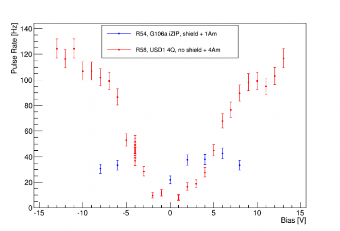 |
The plot above compares Run 54 rates (G106a biased in iZIP fashion) to the current run. Run 54 is the last data in which an internal Am source is used (one source). The Run 58 data shown was taken with no external source present. In Run 54 the lead/poly shield was erected around the fridge, whereas in Run 58 the shield was not present.
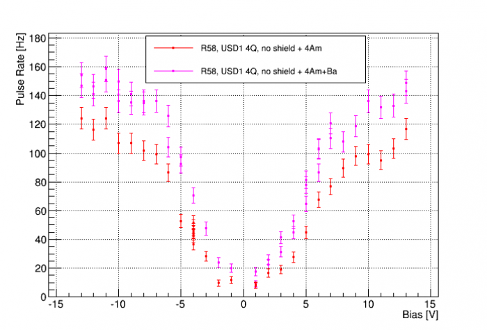
It is surprising that the rate varies strongly with bias. It suggests that the noise threshold, which should be low (note the same threshold is used for both runs) is actually high enough in terms of energy to eliminate a large part of the spectrum at the lower biases. This could be a hint that the charge collection efficiency in USD1 is very low, that the carrier lifetime is short because of a high trap density.
| Event rate versus detector voltage bias in Run 58, comparing Ba runs and no-Ba runs |
|---|
 |
Energy spectra
The plots below compare energy spectra from USD1 with spectra from G106a (iZIPv6) taken in Run 54. The spectra are in raw rq units. There are several similarities and differences between the two situations:
- Both runs use Am sources mounted close to Side 1 of the detector (one source for G106a, four for USD1)
- The G106a data was taken with the detector biased in iZIP mode.
- Side 2 of G106a was read out with a DCRC RevC. The other channels shown use DCRC RevC.1.
- For the G106a data the higher bias was on Side 2; for the USD1 data shown the polarity was opposite, high bias on Side 1.
It is important to understand the differences with respect to the bias layout. First note that the 60 keV gammas from the Am source have a mean free path of only 0.4 mm in Ge, so they will interact close to the surface. In iZIP mode the charge carriers from near-surface events will mostly be collected on the near-side interleaved electrodes with few or no charge carriers drifting to the opposite side. We have seen in the iZIP data that most 60 keV events are such one-side events but there are also some two-side events, events in which the charge carriers drift through the full width of the detector. There are also hybrid events in which some charge is collected on the near side and some drifts to the other side. It is easy to distinguish these types with charge symmetry cuts in the iZIP data (this is of course why the iZIP was developed, for the ability to distinguish near-surface events).
To make a proper comparison the G106a spectra below make no use of charge symmetry. But the iZIP biasing produces some significant differences. On Side 1 of G106a the 60keV line is very prominent, since the full charge will be seen for both one-side events and two-side events. On Side 2 the peak is much smaller because only two-side events are seen. If the bulk charge collection efficiency were high, you would expect USD1 to show a peak similar to that seen on Side 1 of G106a because without interleaving there is no loss of signal as is seen on G106a Side 2.
Note that there is a low-end shoulder in the 60keV peak seen on G106a Side 1. This shoulder disappears if you select only two-side events using a charge-symmetry cut. The shoulder is likely an indication of the “dead layer” effect, the reduced charge collection seen for interactions very near the surface.
For the USD1 spectrum shown a positive bias is chosen (higher bias on Side 1). This should if anything produce a cleaner 60keV line because these will be hole events, i.e. the holes will drift from Side 1 to Side 2 and thus produce most of the signal. Since holes travel straight along the field lines whereas electrons spread out in a cone, the hole events should appear almost entirely on the channel that the Am source producing the gamma is aimed at, rather than being “shared” among multiple channels. The plot shown is for the innermost USD1 channel.
In the G106a data the calibration factors for Sides 1 and 2 differ significantly. This is almost certainly due to the difference in DCRC version (although I don't know the relative amplification factors offhand). Since RevC.1 DCRCs were used with USD1 the calibration should be comparable to G106a Side 1.
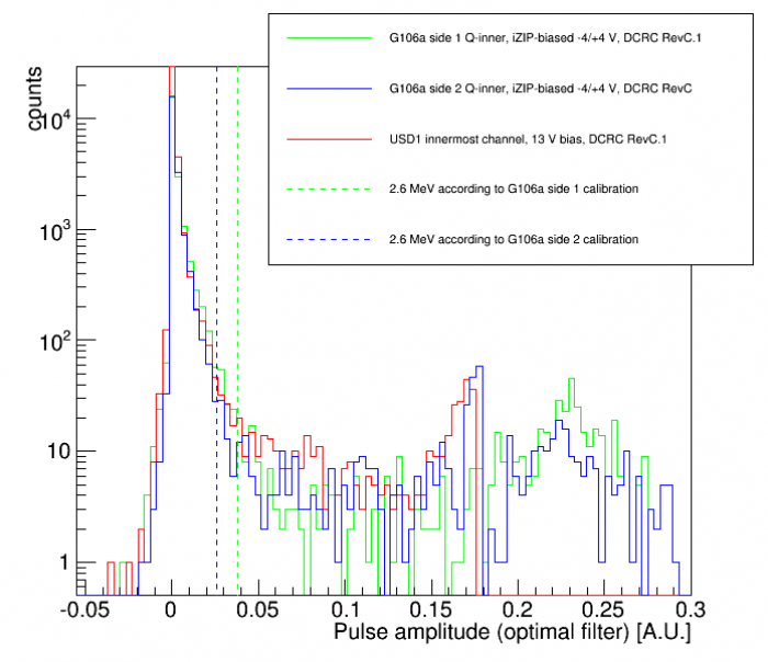 | 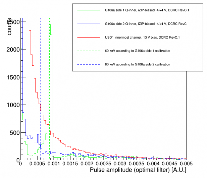 |
| In each case the only cut applied is one to remove randoms. Each represents about 30 minutes of data. | |
The left plot shows the full range of energies. Dashed lines indicate the position of 2.6 MeV for the two G106a charge calibrations, which is the high end of the U-Th background - above this should be mostly muons. The USD1 spectrum cuts off at high energy sooner than the others. At these high energies the charge pulses are generally saturated but I'm not sure why the USD1 cuts off before the others. There are some differences in processing, e.g. different templates were used, but they weren't very different so I don't really understand this.
The right plot zooms in to lower energies. Dashed lines indicate that position of the 60 keV lines for the two G106a charge calibrations (which were calculated using charge-symmetric events).
Why is no 60 keV line seen in the USD1 data? Note that the continuous part of the spectrum in that region is much higher than in the G106a data. The rate is indeed higher but it's not clear that the spectrum for a single channel should look like this. What would be expected is that the 60 keV events would be well-localized to the individual channels, i.e. a gamma from one of the four sources should make a large pulse in the channel it's aimed at and only small pulses in the other channels. So I would expect the additional Am sources would only elevate the very low end of the spectrum. An attempt was made to use partition cuts, i.e. select only events in which the innermost channel is the prominent one, but it does not help. In fact the partitioning pattern in the detector is confusing - more events seem “shared” than I would expect. This should be studied further and compared with other 4Q results.
Perhaps the 60 keV line is smeared out due to poor resolution. Perhaps the dead layer is rather thick so that all 60 keV events are in the layer and therefore strongly attenuated.
analysis plan
Run 58 (USD detector)
claim: something is wrong with this detector, as compared to most same-size CDMS Ge detectors
reason: cannot see 60 keV peak
Things to compare
- spectra
- best if not interleaved
- rate
- noise
- new run (Run 59) - will hopefully provide more, better comparison data
Things to measure
- try using spectral shape to characterize relative efficiency
- at different biases
- over time in a series (deneutralization)