Table of Contents
Run 70 Summary
Data series listed here: DataSeriesList.xlsx
SQUID Temperature
HV Noise
0-Volt Noise and Noise Per Channel
In general, using balanced PsumOF, the 0-Volt noise sigma for this run is 650-700 eV.
This is much higher than we achieved in Run 66: around 280 eV.
One theory for the difference is that the higher temperature now (40 mK versus 20 mK in Run 66) results in significantly lower TES gain, dI/dP. Our 0-Volt noise is current noise (passive Johnson noise), and as shown below it seems to be the same in this run as in Run 66. But since it is current noise, lower dI/dP means that the noise in energy units is higher (so really it's reduced signal-to-noise).
5/30/19
For the data collected on 5/30/19, each individual channel was looked at. Plots were made for each channel showing the fraction of energy in that channel vs energy. Each plot showed a line at a specific fraction that was different for each channel. In order to match the channels to each other, factors were found for each channel such that when you multiply the fraction for each channel by its respective factor you get 0.1. All channels were then multiplied by their respective factor and added together then calibrated to eV. It was found that the width of the 60 keV peak was slightly smaller for Psum than for PTOF.
| Width (sigma) of 60 keV line (in keV) | |
|---|---|
| PTOF | Psum |
| 1.975 +- 0.004 | 1.893 +- 0.006 |
Using the calibration and the individual channel factors, the 0-Volt noise was found on each channel.
| Channel | Noise (in eV) |
|---|---|
| A | 171 |
| B | 157 |
| C | 595 |
| D | 257 |
| E | 339 |
| F | 155 |
It appears that channel C contains significantly more noise than the other channels. When added in quadrature, the total noise was 782eV. The 0-Volt noise on PTOF was 711eV and on Psum was 860eV.
5/29/19
The same process was done for the data collected on 5/29/19 with a different set of biases.
| Channel | Noise (in eV) |
|---|---|
| A | 187 |
| B | 171 |
| C | 365 |
| D | 286 |
| E | 314 |
| F | 202 |
0V Noise Spectra
Below are example PSDs from this run and Run 66 for comparison. There are a few notable structures in PA in Run 77 and PC in Run 66, but the noise levels and shapes are otherwise similar.
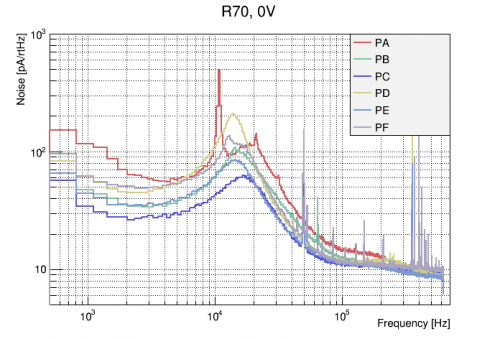 | 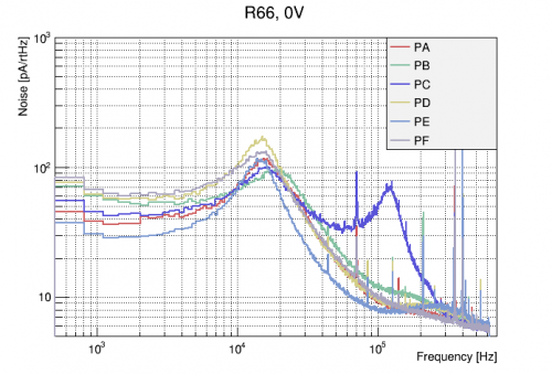 |
| R70 0V Noise PSDs | R66 0V Noise PSDs for comparison |
|---|
The superconducting spectra are are also shown below. All channels show behaviour similar to that in R66, with Passive Johnson Noise levels of ~60 pA/rtHz. The pole of PC appears quite high and is associated with strange, “drippy” electronics noise on this channel when QET bias is set to 0. This noise does not appear at small, non-zero QET biases.
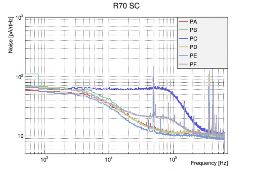 |
| R70 Superconducting PSDs |
|---|
| Channel | I_PJN,SC(0) [pA/rtHz] |
|---|---|
| A | 55.5 |
| B | 64.5 |
| C | 62.8 |
| D | 63.8 |
| E | 54.5 |
| F | 60.6 |
| Avg | 60.3 ± 4.0 |
Data quality issues
Detector activation planning
In order to provide Ge activation lines, we are planning to activate the detector with a PuBe source located inside the shield, assuming that we want a 1 keV line as strong as Am 14 keV line. Estimated time of exposure,  , is calculated to be 1548.28 seconds or 25.8 minutes; time of exposure will be 26 minutes. Calculation via the expression,

where  (is a component of
 ),
 ,
 , and
 . All constants should have the same units (minutes or seconds).
Update: our standard 180V data with phonon thresholds set to 6 has a very low write efficiency, estimated at around 25% (trigger rate is probably close to 270 Hz). So the rate of 14 keV events is higher than we thought, 0.08 Hz rather than 0.02 Hz. This suggests a desired exposure time closer to 4 hours.
Unbalanced Energy Calibration
It was seen early in this run that unbalanced amplitudes, with for example deweighted inner-ring channels, produce significantly better noise widths than balanced quantities. The extreme case is a calibration based on a single channel (e.g. pF, the center channel). Here we explore this in some detail.
pF-only calibration
A look back at Run 66
Exploring balanced and unbalanced calibrations in Run 66. This breaks down the contributions of each channel to the noise, shows that the noise from the channels is partially correlated, and shows that any one channel produces a better resolution than a combination of channels.
Summary
In both Run 66 and this run, the best noise sigma achievable with a balanced total phonon quantity is around 40 eVee.
In both runs, we can do significantly better with a pF-only quantity and a tight fiducial cut: 18 eVee in Run 66, 11 eVee in this run. (Vdetector around 70V in the Run 66 data, 130 V in the Run 70 data).
This suggests that the vacuum interface has not substantially improved the noise performance. It's possible that we're able to get to higher bias in this setup - that may have more to do with the change in wiring.
(n,gamma) Signal Rate
The plot below shows Anthony's simulated (n,gamma) NR spectrum for germanium, for events in which the gamma escapes the detector without interacting.
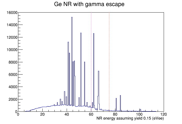
This spectrum has no resolution smearing - the observed spectrum may be very smeared out. There's some question of whether we can expect to see sharp features.
We can estimate the rate at which we should see (n,gamma) signals using Anthony's simulation. Here are the steps in the calculation:
- From Run 66 we found that with the PuBe source in the standard place, the rate of neutron captures on 70Ge in the detector is 1.38 Hz
- Considering the different abundances and capture cross-sections of the five Ge isotopes the total neutron capture rate in the detector is 4.55 Hz
- The simulation is for a total of 1073996 (n,gamma) events
- Therefore the total time represented by the simulation in our standard setup is 65.6 hours
- Assuming Y=0.15, the total number of simulated events above 60|75 eVee is 44620|11442
- Therefore the rate of signal events above 60|75 eVee is 681/170 events/hour
- In Run 68 our total signal efficiency after cuts and DAQ event loss was about 40%
- We can hope for a duty cycle around 50%
- With these efficiencies, with threshold 60|75 eVee we would expect 3269|816 events/real day
- Let's suppose an additional single-channel fiducial cut with efficiency 10%
- Then with threshold 60|75 eVee we would expect 327|82 events/real day
- If we want a minimum of 1000 signal events, at threshold 60|75 eVee it would take 3|12 real days
Trigger Optimization
Write Efficiency
We compared write efficiencies and event rates over different kinds of data. The data sets that we looked at include:
- bkg (earlier): background data 07190813_1156→07190813_2231, trigger threshold = 6
- bkg (later): background data 07190819_1824→07190820_0646, trigger threshold = 6
- bkg thresh=7 : background data 07190820_0942→07190820_2017, trigger threshold = 7
- bkg thresh=8 : background data 07190821_1108→07190821_2330, trigger threshold = 8
- PuBe : PuBe data 07190726_2304→07190727_0929, trigger threshold = 6
- Na lower : Na data at lower rate 07190814_1502→07190815_1200&07190815_1909→07190815_2032, trigger threshold = 6
- Na higher : Na data at higher rate 07190816_1004→07190817_0708, trigger threshold = 6
The efficiencies and rates we evaluated include:
- write rate: the rate of written events in triggered data
- true event rate: the rate of “triggerable” events, inferred from “hits” in randoms
- write efficiency of triggered data
- write efficiency of in-run randoms
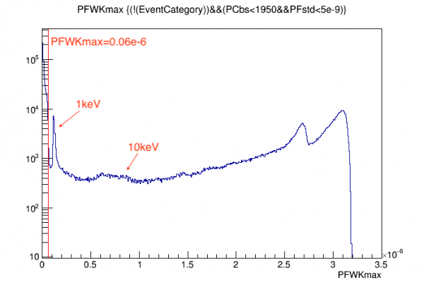
For each case, an event was defined with pulse-hight threshold “PFWKmax > 0.06e-6”. As an example, below shows the spectrum for some of the bkg data series, and events are what's on the righthand side of the vertical red line. Identifying 10keV peak and 1keV peak, we can know that the threshold approximately corresponds to ~0.7keV.
| True Event Rate (Hz) | Write Rate (Hz) | Write Efficiency (triggered data) | Write Efficiency (in-run randoms) | |
|---|---|---|---|---|
| bkg (earlier) | 30.2 ± 0.7 | 27.1 ± 0.4 | 89.5% ± 2.6% | 40.9% ± 0.7% |
| bkg (later) | 30.3 ± 0.5 | 25.1 ± 0.4 | 82.8% ± 2.0% | 69.9% ± 1.2% |
| bkg thresh=7 | 32.7 ± 0.5 | 23.9 ± 0.4 | 73.0% ± 1.7% | 92.1% ± 1.6% |
| bkg thresh=8 | 30.9 ± 0.5 | 23.3 ± 0.4 | 75.6% ± 1.7% | 93.4% ± 1.6% |
| PuBe | 77.9 ± 1.7 | 36.1 ± 0.6 | 46.3% ± 1.3% | 17.7% ± 0.4% |
| Na lower | 77.4 ± 1.8 | 39.4 ± 0.6 | 50.9% ± 1.4% | 18.6% ± 0.3% |
| Na higher | 120.9 ± 1.8 | 40.5 ± 1.6 | 33.6% ± 1.4% | 19.0% ± 0.8% |