Table of Contents
Run 54 Summary
first_tests_of_hv_board_for_izipv6.pptx hvboard-first-test.pdf izipv6-at-umn-with-filters.pdf izipv6-at-umn-with-filters.pptx
UCB analysis note on HV test of 3" iZIP
Noise PSDs at various Front-end Gain settings
Noise PSDs at various TES states
Noise PSDs at various TES states, with and without filters (20ms traces)
Noise PSDs with different DCRC arrangements (20ms traces)
Noise PSDs at various HV settings
| Phonon spectrum, 2015 Sep 1 -4/+4 V |
|---|
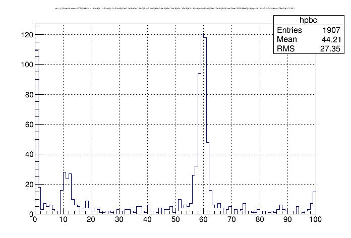 |
| cuts: charge symmetry, randoms removed. No quality cuts. |
| channel balancing factors individually set to 0.5, 1.0, or 2.0 to minimize 60keV line width |
| empirical ptotal calibration. |
More preliminary looks at iZIP-mode data
Strange results trying to create PSDs, compare with cdmsbats results
HV tests
Matt Pyle's summary:
- Remove LEDs from consideration by grounding them
- make sure that when the TES are superconducting we don’t see a TES current change that correlates with bias voltage shift
- See if you can see shot noise in the TES noise … if not, prove that you shouldn’t be seeing shot noise by doing the calculation, and showing the quanta is too small
Results:
LED grounding
All LEDs were grounded in the HV box on 20150914. No significant change in behavior in terms of leakage or heating/breakdown.
Current leakage into QETs
We applied 0 QET bias to two channels on 20150914. We increased the HV and watched for changes in the baselines. None were seen - except that when they were driven to normal they shifted, which they shouldn't have. This is interpreted as an offset to the QET bias of a few μA so that they weren't actually set to 0.
I expect that in this procedure the resolution for current change in the QET is around 10 nA, so leakage is less than that. That value is comparable to the full leakage in the HV board so it's clear that there is not much sensitivity. It's also clear that this small amount of current can't heat the QETs.
Quantifying breakdown
V_crystal versus V_luke
We have been calculating the voltage on the crystal as Vcrystal = Vsupply - Rbias*Ileakage. The main bias resistor is 400 MΩ but there are also 40 MΩ resistors on each of the 14 lines biasing Side 2 of the detector. So depending on where you think the leakage is occurring, Rbias could be between 400 and 440 MΩ. At one point I decided on 430 MΩ because it made positive and negative data more consistent. (Correction: see this correction in the Run 57 summary.)
Matt Pyle found that the crystal voltage calculated based on leakage was different from what was implied by the apparent Luke gain. You can find the Luke gain from phonon data if you compare a phonon spectrum at a given HV setting to a phonon spectrum at 0 bias. The ratio of the calibration factors (from raw phonon signal units to keV) gives the Luke gain, from which you can calculate the effective Luke voltage.
Data taken on 20150908 at four different HV settings was processed and analyzed. Removing randoms but neglecting quality cuts, 60 keV peaks are visible in the phonon spectra based on integrated pulse quantities. Peaks were seen in HV1pA, pB, and pC (Side1 channels B, F and C) so these were summed.
| Fits of 60 keV phonon peaks at different HV settings |
|---|
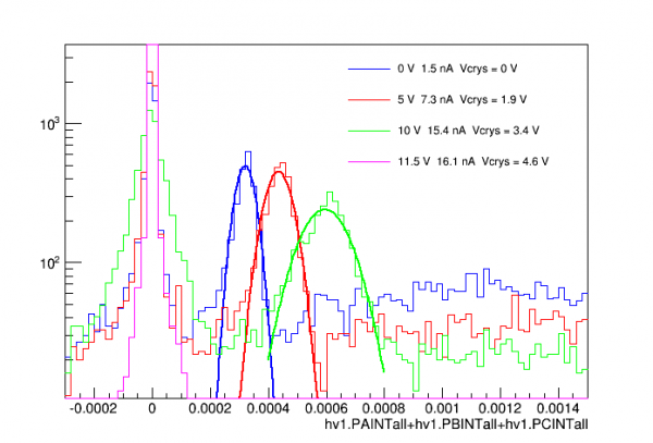 |
| note: at the highest HV setting (magenta) the TES's were driven close to normal resistance |
The gains for the non-zero bias cases can be calculated by dividing their peak positions by the zero-bias peak position. From these gains one should be able to calculate the voltage:
G_luke = 1 + V_crystal / [3.0 V]
The voltages derived this way are significantly smaller than what is estimated from the HV setting and leakage current measurement and an assumed Rbias between 400 and 440 MΩ. However at these low voltages we know that the charge collection efficiency is much less than 100%. Reduced charge will also mean reduced Luke gain, so that
G_luke = 1 + q_efficiency × V_crystal / [3.0 V]
In run_39 the charge collection efficiency was measured for G106a. If we apply +V to Side 2 in HV mode, it is equivalent to -2V/+2V in iZIP mode, which is the left side of the plot below:
| Charge collection efficiency measured in Run 39 (iZIP mode, symmetrical biases) |
|---|
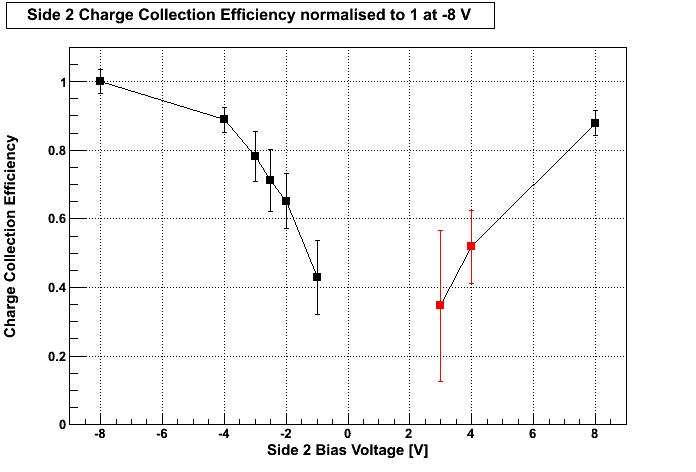 |
If we assume that the voltages as calculated from the HV setting and leakage are correct (using Rbias = 430 MΩ), it implies that the charge collection efficiencies for the HV=5V and HV=10V cases are 58% and 76% respectively. This corresponds to voltages on the crystal of -1.9 V and -3.4 V, so it can be seen that these efficiencies are consistent with the seagull plot results.
The conclusion is that V_crystal = V_HV - I_leak × [430 MΩ] is approximately correct.
Quantifying breakdown from shifts in phonon baseline
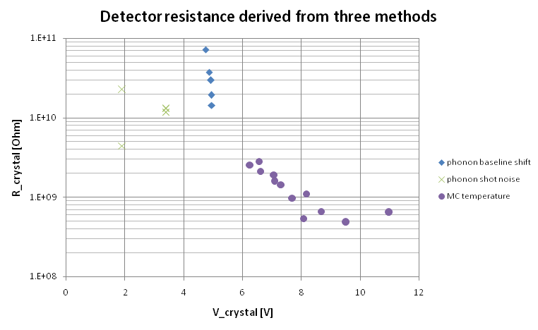
On 20150915 and 20150916 we increased the HV setting until the phonon baselines began to change, then measured the baseline of HV1pA as a function of crystal voltage:
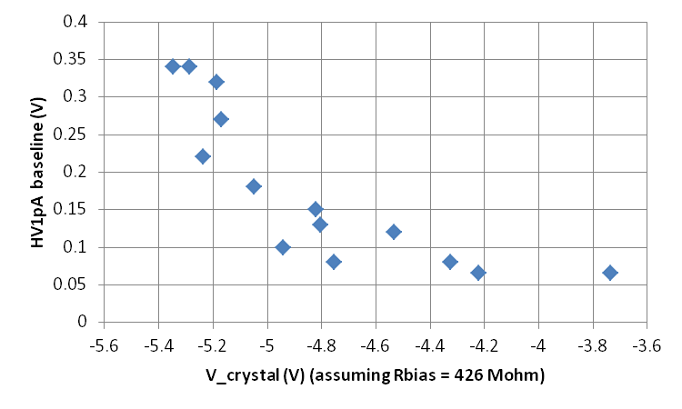 | 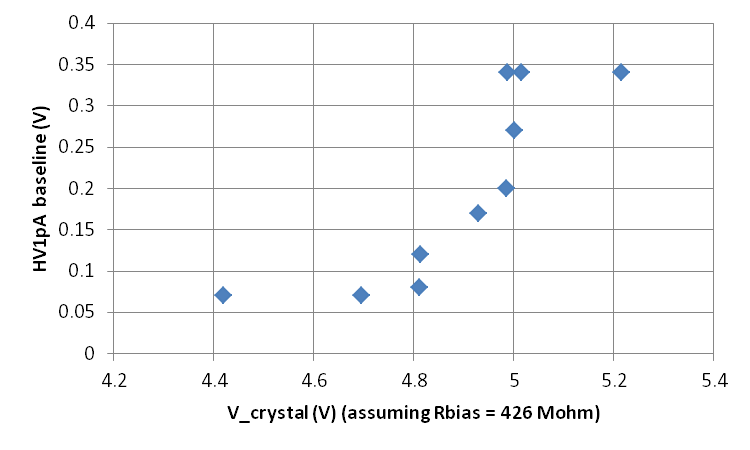 |
If we interpret the shifts in baseline as due to increasing power being absorbed in the TES from phonons produced by conduction through the crystal, we can use the results above to infer the total power dissipated by the conduction and, knowing the voltage on the crystal, calculate the apparent resistance of the crystal. To do so we must estimate what fraction of the total power is absorbed by the TES. In the Run 53 summary I estimated the phonon_collection_efficiency for G106a to be 12.4%; here I make the further assumption that a single channel receives 1/12th of this, for a single-channel collection efficiency of 1.03%. The resulting resistances are shown below:
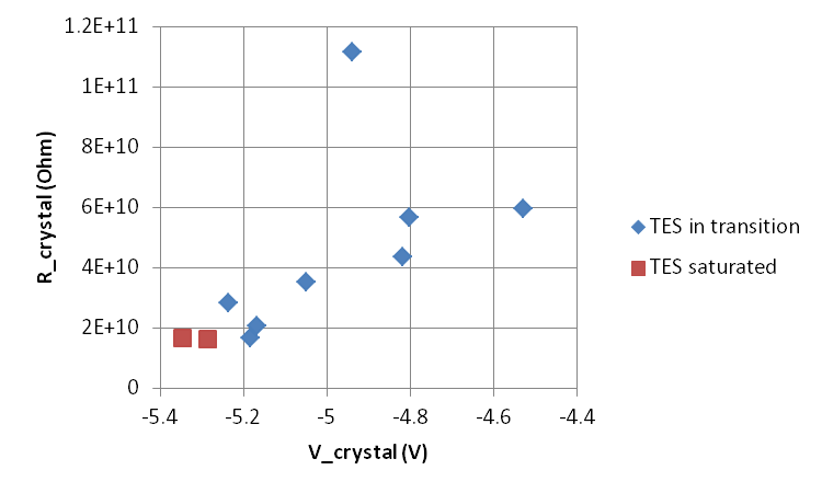 | 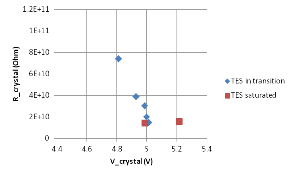 |
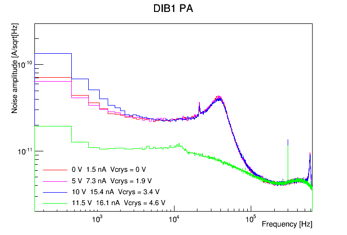
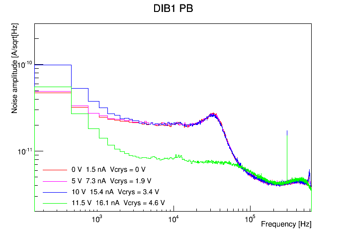
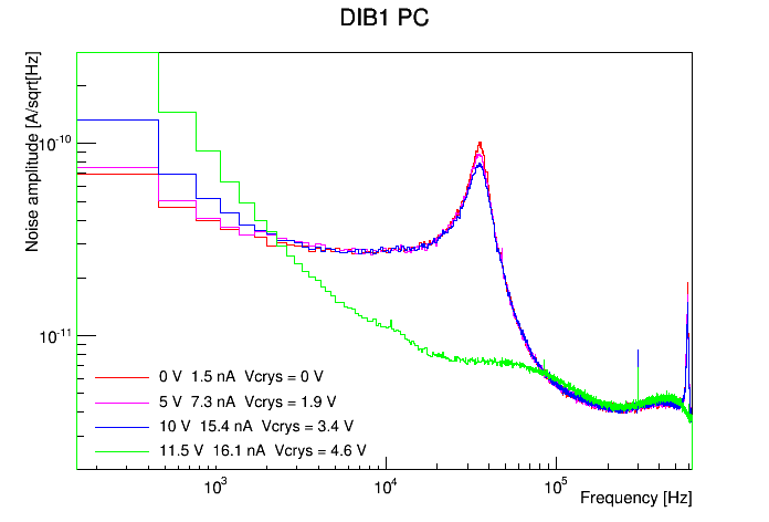
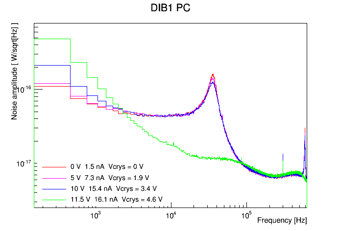
From the data taken on 20150908 at four different HV settings we also looked at noise PSDs. A rough pulse-removing cut was applied to the 1000 randoms in each case (standard 4 ms traces):
| Current noise PSDs at various HV settings | ||
|---|---|---|
 |  |  |
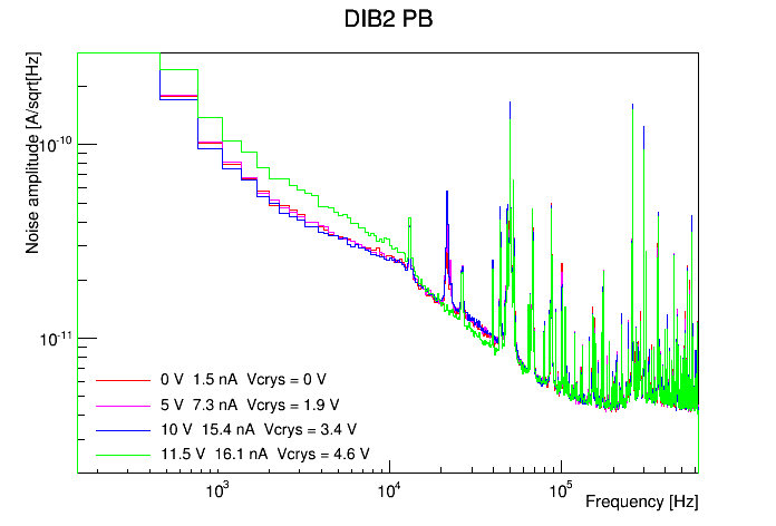 | 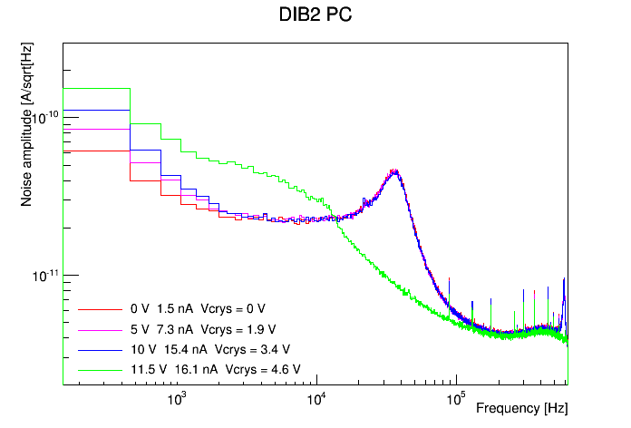 | 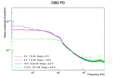 |
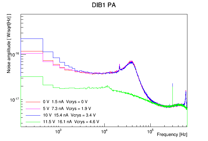
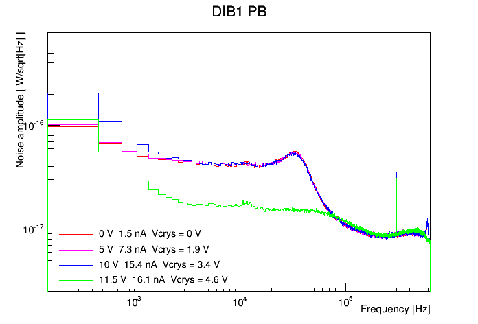
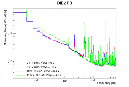
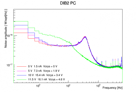
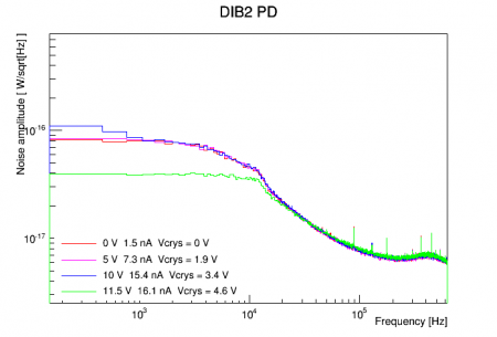
The PSDs above were converted from A/rtHz to W/rtHz by multiplying the amplitude by the TES voltage. The TES voltage was calculated as the QET bias current multiplied by an approximate parallel shunt+TES resistance of 18 mΩ:
| Power noise PSDs at various HV settings | ||
|---|---|---|
 |  |  |
 |  |  |
In UCB analysis note on HV test of 3" iZIP Matt Pyle derived the shot noise one would expect to see in a TES produced from a current through the crystal, taken to be individual charge carriers (or pairs) Poisson-distributed in time, each producing a pulse of Luke phonons. His formula frequency-dependent formula is
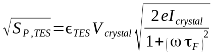
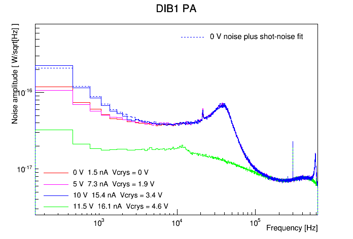
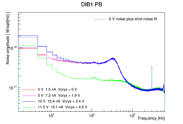
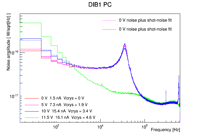
The power noise depends on the voltage and current through the crystal, the TES phonon collection efficiency, and the bandwidth characterized by the phonon pulse fall time τ_F. The results here can be expected to differ from the Berkeley results in that the voltage is much smaller and the pulse fall-time is larger - about 900 μS for G106a - so that the shot noise PSD will fall off at relatively low frequencies. Using this formula I attempted to fit the power noise spectra to a model of noise-at-zero-volts plus shot-noise (added in quadrature). Below are the power noise plots with the added fit shot noise shown as dashed lines. I omit the fits where it seems to fail or is inapplicable.
| Power noise PSDs at various HV settings with shot-noise fits (dashed lines) | ||
|---|---|---|
 |  |  |
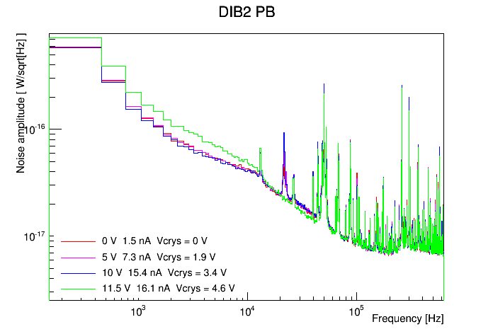 | 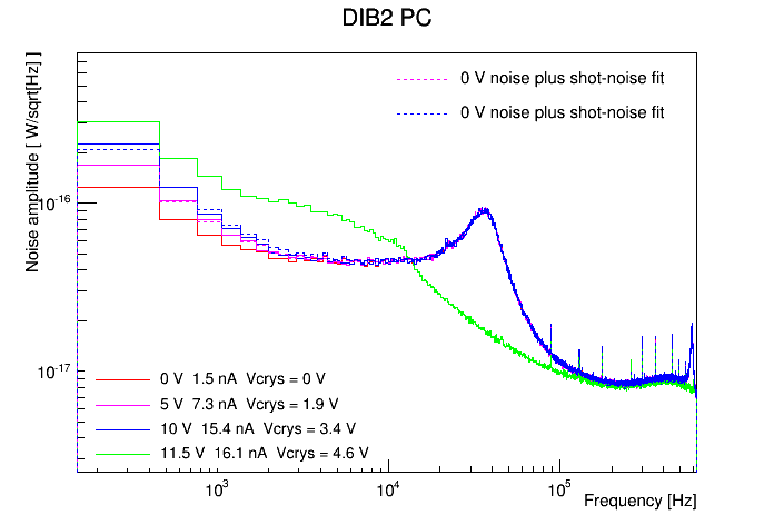 | 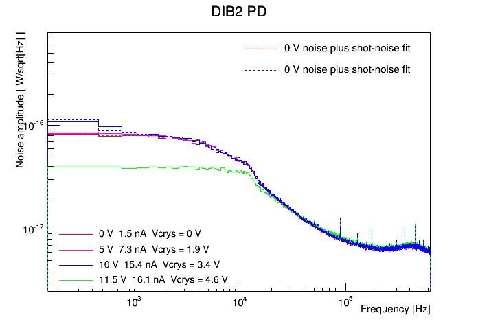 |
The shot-noise fits are not very good in terms of their frequency dependence, which was also the case in the UCB note. I performed the fits assuming a fixed pulse fall-time of 900 μS, with the current as the only free parameter. (Attempts with the fall-time as an additional free parameter resulted in either failed fits or implausibly high fall-times, over 20 ms). Using this current we can calculate the effective crystal resistance. Each channel gives an independent measure for the current at each non-zero voltage setting. Performing this calculation for the good fits shown above, it seems that DIB2 pD is an outlier - this channel seems to be behaving differently - so I leave it out in the plot below:
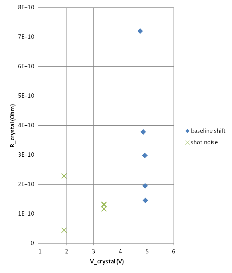
The resistances for V_crystal=1.9 V are not very consistent with one another, but the four resistance measurements from the channels used at 3.4 V are in good agreement with one another and seem to agree with the lower values calculated in the baseline-shift study, around 12 GΩ.
Relative coverage of the phonon channels
In processing we make use of the relative coverage of the phonon channels in order to calculate the “relative calibration” (i.e. to scale each channel's amplitude so that a scaled amplitude represents the same phonon energy for each channel). This is done with late-pulse data under the assumption that late in an event the phonon flux is uniform throughout the detector. The late-pulse amplitude divided by the coverage for each channel should be equal after scaling.
Originally we assumed that info on the Confluence page for iZIPv6 concerning the area of the region occupied by each channel:
Phonon sensor areas should be: A = pi*50^2 - pi*44.8^2 = 1550 B,C,D,E = (pi*44.8^2 - pi*19.2^2)/4 = 1287 F = pi*19.2^2 = 1158 mm^2
gave the relative coverages. But this is only true if the phonon-sensitive area of a channel (namely the area of the Al fins of all the TESs) represents the same fraction of the areas above for every channel.
After an email exchange with Paul Brink and Matt Cherry I came to the conclusion that the Al fin coverage is the same for every TES, so the number of TESs per channel would give us the relative coverages. But apparently nobody knew how many TESs per channel. There were some vague ideas. Images on the Confluence page were detailed enough so that you could count the TESs manually. I attempted this but it was particularly arduous for the outer channel (Channel A) because the TESs are close-packed with no space between them - you need a tight zoom to distinguish them. See file below:
Counting TESs on iZIPv6 mask diagram
My conclusion is that the 5 inner channels (B-F) each have 458 TESs. The outer channel (channel A) has around 455 TESs.
Matt Cherry was able to query the mask file to find 2748 instances of the TES unit cell on the mask, which is equal to 458*6. So most likely all six channels have the same coverage. There may have been changes to add additional bonding pads. I'm awaiting confirmation.
The current conclusion is that the channels have equal coverage, contrary to what we'd assumed previously based on the areas of the channel regions.
Breakdown problems in high bias runs
When we started taking overnight bias-sweep data, from -8/+8 V to +8/-8 V, we found that the noise was very dependent on the bias:
Noise PSDs with different charge biases
Looking more closely at bias-scan running during the day we realized that we are getting charge breakdown symptoms at the higher biases. In our most recent charge breakdown study we found breakdown at high-ish biases that could be avoided by overshooting the bias to maximum then backing down to some desired value. Using noise PSDs as a figure of merit we did some noise tests to determine at different biases whether it is important to overshoot the bias before setting the desired bias. We also checked to see whether flashing beforehand was relevant.
With DAQDAQ in standard overnight running the biases are set to zero and the detector is flashed, then after cooldown when a new series starts the bias is increased to the desired setting. When we took the noise tests we also tested whether flashing beforehand is relevant. During the tests it appeared that only the positive-biased side needed to be overshot, so in the series labelled “overshoot” only the positive side was overshot.
The test results are here: PSDs at various biases with various pre-biasing conditions.
Observations:
- It seems that both overshooting the positive bias and not flashing can improve the situation. Not flashing however is not really an option - we need a neutralized detector.
- Overshooting the positive bias improved noise in all channels -6/+6 V and +8/-8 V
- Overshooting the positive bias improved noise in some channels at +6/-6 V
- Overshooting had only marginal improvement at -8/+8 V. It may be that the TESs were being driven normal or near-normal in the overnight runs which overall improved noise but of course would have a bad effect on resolution.
Operationally speaking, we have decided that data with biases greater than 4 V will only be taken during the day, when we can “manually” overshoot the positive bias before beginning the series. (One has to wonder whether our many -4/+4 V series may have been improved by overshooting, but hopefully there is no breakdown at so low a bias.)
MIDAS status
from an email from Anthony dated 2015 October 22:
MIDAS core data acquisition code
We can take data in the same way that Berkeley has taken data with this. We can view and save pulses from a file. If there is interest, we can switch over to doing all of our PSDs like this. But I don't see a real need at the moment because the when we get the processing running you can just do it the same way (either use the filter files or BatViewer).
Amy and I have developed the ability to produce files in the same naming/directory format as we're used to.
I have developed the ability to take a string of beginning-of-run and end-of-run random triggers.
What remains is to be sure that we're getting appropriate triggers from DIBs 2,3 and that they are in-sync with our other DCRC. And also to be able to process the data in the output format given, or convert it to the standard SuperCDMS data format. Then we have to test that. This job is a week ish timescale, but it depends on the paradigm I choose for the solution a little.
After doing what needs to be done in the last paragraph, we can take data with MIDAS and analyze it properly.
DAQ tuning tools
In the MIDAS paradigm we have a tuning tool that can be used to tune SQUIDs etc. I installed this and it works. David has used it, and it's been tested and behaves not much different from the LabView interface currently. We can move to use this exclusively at any time.
I am listed as a person who will develop a IbIs script in this framework. That might be the only thing we don't have already going that you guys use. Of course you could still do it the “old” way. Anyway, this job is lower in priority than the above MIDAS development but is still high on the to-do list. If someone wants to learn the DAQ interface/detector tuning tools better, they can help with this.
DAQ UI and sequences
I have developed a flash and ZAP sequence that have been tested successfully. These are implemented as part of the DAQ code, they are python scripts that Allison and Nick should be able to understand/modify with a small amount of starting guidance. David should be brought up to speed on these, so he can modify them as he pleases if there is a specialized “sequence” that you'd like to do.
Amy has created a nice DAQ UI for interaction with detector settings that provides a more visual interface than directly changing the ODB on the MIDAS frontpage (http://jiajin.spa.umn.edu:8081). She added to those support of the flash and ZAP sequence so that those are both currently at the level of “push a button” to have them work. This has been tested.
I will implement a flash-and-take sequence. It won't take much work and perhaps I can work closely with Allison/Nick/David on this so that they are familiar with what needs to be done. We will connect it to Amy's frontend too.
Problems with He recovery
The monthly He gas recovery rate for the K100 lab has been decreasing:
| Month | Liters used | Recovery rate |
|---|---|---|
| March | 610 | 94% |
| April | 220 | 90% |
| May | 645 | 76% |
| June | 771 | 81% |
| July | 632 | 85% |
| August | 617 | 69% |
| September | 685 | 85% |
| October | 753 | 84% |
There are two issues here:
- Starting in May recovery dropped significantly. This coincides with Matt replacing Hassan and it's likely that Matt's faster&rougher transfer style has made recovery during transfer less efficient.
- August recovery was very low, suggesting some new problem with the system that needs to be investigated.
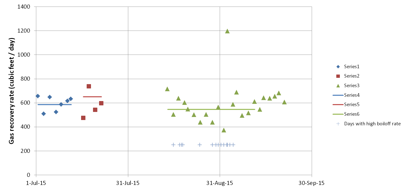
There are some observations that may be clues about the August problem. First, faster boiloff rates have been occasionally observed during Run 54. The problem is sporadic - sometimes it's around 20% higher than normal, sometimes it's normal. Second, looking closely at the overall rate during a run at which gas is being recovered (data from the transfer log) shows some patterns:
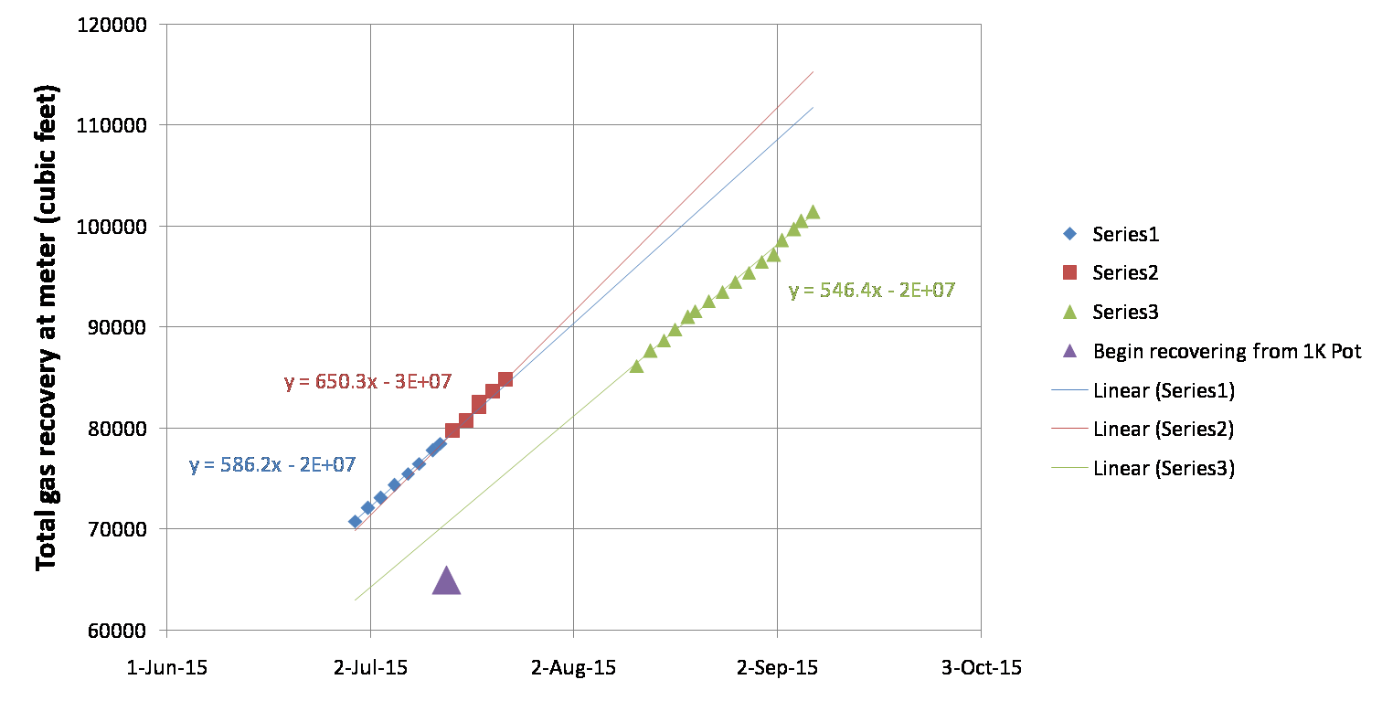 | 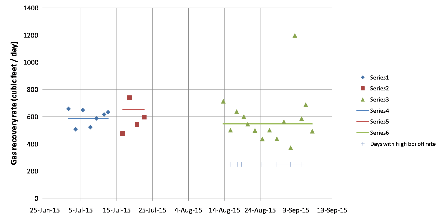 |
The overall rate of gas recovery while cold increased after we started pot recovery by 11%. But after the warmup and cooldown between runs 53 and 54 the rate dropped by 16%. The second plot is to look for short-term trends and some correlation between the low recovery rate and the periods of high boiloff rate, but it's difficult to see any trends in the noise.
Remediation
For the problem of severely low recovery fraction in August, Paul Crowell suggested that the most likely cause would be a leak in the recovery system. On 2015 September 11 we hand-tightened all of the KF and compression connections in the bath & recovery system. Some were a little loose. We also attempted to Snoop for leaks in various places during a transfer but didn't see anything. If we don't see an improvement in recovery rate over say the next week or so we will look for leaks in more of the system (we did not try the hard plastic joints along the walls and near the meter).
For the problem of generally less efficient transfer after April we are changing the transfer style, reverting back to something closer to Hassan's style. In recent months the overall rate at which the bath filled during a transfer was typically 1.5-2.0%/minute. As of 2015 September 11 we are targeting 1.0%/minute. Also we will not fill the bath as high as we sometimes do: we are reverting back to Hassan's method of stopping Dewar pressurization at 85%, then ending the transfer at 90%. Here are some useful targets during a transfer:
- The “chirp rate” of the meter should be kept around 10 chirps per 12-13 seconds.
- The rate at which the bath should rise after we start pressurizing the Dewar should be close to 1.1%/minute.
As usual the transfer rate can be modulated by adjusting the Dewar pressurization valve, which is generally opened to about 1mm from the closed position.
If there gas leaking from the recovery system during a transfer it would of course be best to fix the leak, but even if leaks are present the leakage should be reduced by doing more gentle transfers, keeping the bath & recovery at lower pressures and preventing it from getting quite as cold.
The occasionally-higher boiloff rates may be a separate issue. It could be that the cryostat vacuum jacket has degraded. We have not pumped it out since before April. To pump it out we will of course need to be warm, but we will also need to remove the shield because the cryostat needs to be dropped several inches to access the port. We should pump it out next time we have the cryostat down.
Update
Since we reverted to more gentle transfers on Sep 11, the daily rate at which He gas is being recovered seems to have increased. In the updated plot below the green points past the green line represent measurements since we modified the technique. The rate seems to be as high as “Series 2”, which represents the period in the last run (Run 53) after we began recovering the 1K Pot exhaust.