Run 53 Summary

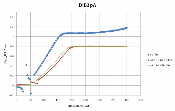
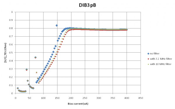
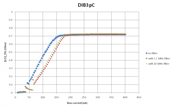
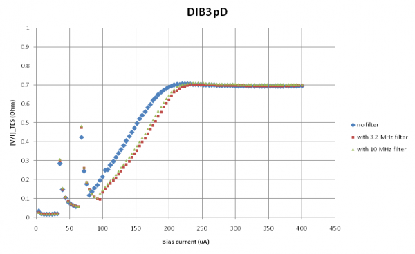
We tested the effect of placing d-sub filters in series with the DCRC - a 3.2 MHz Pi filter and a 10 MHz C filter. We tested the filters on DIB3 with DCRC50 (RevC.1). It was immediately clear that QET biases that worked without the filter were too small with the filter present. Apparently the filter remove an unknown AC component from the bias current, reducing the effective excitation.

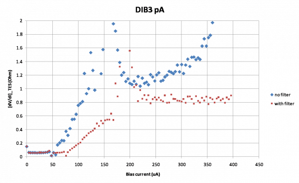
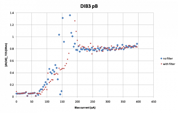
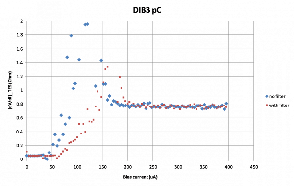
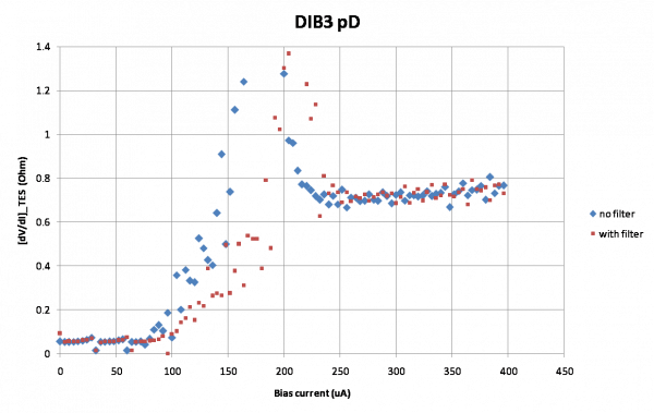
IbIs data was taken with and without the filters. From these we derived resistance (TES plus parasitic) versus I_bias curves, shown below. The general trend is that R_parasitic and R_normal are the same with and without the filter, but the transition is shifted to higher bias current values with the filter present. (Phonon channel A's normal-resistance is an anomaly, with strange behavior in the no-filter measurement. We repeated the no-filter measurement and got similar results.)

The R versus I curves are created from IbIs in two different ways. The top four plots are proper resistances, V/I, for which the offset of the output signal must be derived; these are correct for the transition and normal regions but not for the superconducting region due to the phase-jumping behavior of the SQUID output in this region. The bottom four plots are abs(dV/dI), which requires no offset but only makes sense as a resistance for the constant portions - superconducting and normal - and not for the transition region.

The filters we used were a 3.2MHz Pi filter and a 10MHz capacitive filter (Data Sheet: 3.2MHz: filter designation C and 10MHz: filter designation N). It should be noted that in several places in the run diary, we mistakenly refer to the 10MHz filter as a 100MHz filter. We have done our best to rectify these errors, but we may have missed some.

There were several different issues with data acquisition this run: railing phonon channels, slow event rate, and low frequency noise.

After reviewing data taken using the DAQDAQ2 LabVIEW VI, it was discovered that after flashing, phonon channels were likely to rail, which could sometimes be fixed by changing the Polarity of the phonon channel from Non-Inverting to Grounded and back. If that failed, we changed the Driver Offset to see if we could revive the channel.

DCRC31 also exhibited its own unique problems in addition to the railing channels: Upside down pulses, non-responsive LEDs, and shifting QET biases. In addition, seemingly randomly DCRC31 would go into a “bad state” where a strong noise would appear on the charge channels (the kind observed when the FET is unpowered) and the fridge temperature would rise. Once in this state, the board seemed to become unresponsive and would not obey commands necessitating a power down followed by ~30 minutes before repowering the board. The waiting time was determined empirically.

It was eventually discovered that we could take data without railing phonon channels (as often) by using MultiDAQv3 VI instead of using DAQDAQ2 to automate the process. Flashing manually and keeping DCRC settings the same (except for Q-bias) throughout several runs/flashes allowed multiple data sets to be taken. The suspicion is that sending many commands to the DCRCs does something internally to shift the baseline of the phonon channel, causing it to rail. More investigation into the VIs will take place to see if they do in fact write less-frequently to DCRCs when settings stay the same from run to run. The working procedure is detailed below.

Procedure for data taking (from voltaged state)

  1. Use Detector Control VI to set the voltages to zero on DIB 1 and DIB 2
  2. Use the putty sessions to turn on the working sets of LEDs for 30 seconds
  3. Observe the temperature spike to around 220mK and wait to get within 1mK of target on cooldown
  4. Use Detector control to set the voltages to the correct values
  5. Start data using MultiDAQ and be sure all phonon and charge channels that should be there are there
  6. Wait until the randoms end (event 1000) and start a timer for 15 minutes
  7. When 15 minutes is over stop the run on the MultiDAQ and repeat

It was observed that using an electric pencil sharpener, which had been plugged into a “dirty” outlet, corresponded to a massive railing event across all 3 DIBs. The DCRCs are powered by adapters plugged into a “clean” outlet. Measuring the grounds of the two types of outlets, it was found that they were connected. Whether this is a fault with the building design or because we are connecting them inadvertently, this could be one of the things contributing to odd DAQ behavior.

At several times during data acquisition, the event rate would drop from its typical ~15Hz to ~2Hz, and the computer's memory/CPU usage would spike with LabVIEW contributing most of that. Stopping MultiDAQ VI would immediately bring the CPU usage back to ~15%. It was found that placing a source nearer to the detector would cause the rate to drop as did setting the Phonon Trigger Thresholds in Detector Readout VI too low.

Attempting to take randoms with QETs in superconducting state, caused the event rate to slow after getting through a certain percentage of the pre-run Random Triggers For a setting of 1000 Random events, the computer bogged down around 830 events. When set to 100 randoms, it bogged down at ~60 events. Set to 5000 randoms, it got past 1000 but then hit a “not enough memory error” some time later, which necessitated halting LabVIEW via Task Manager.

We tried clearing up disk space, restarting LabView, rebooting the computer, going back to biased QETs, but the problem persisted. After power cycling the DCRCs for whatever reason, we tried once again to use MultiDAQv3 to take data, and the issue was fixed.

When taking background data with only one DCRC powered, we achieved a data rate of ~25Hz, which is the fastest we've seen in recent memory.

An oscillation of ~175Hz was seen frequently in the pulses throughout the run.

Sometimes, railed phonon channels would cause a ~6kHz oscillation in the charge channels. Relocking the phonon channels would remove the oscillation.

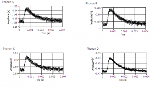
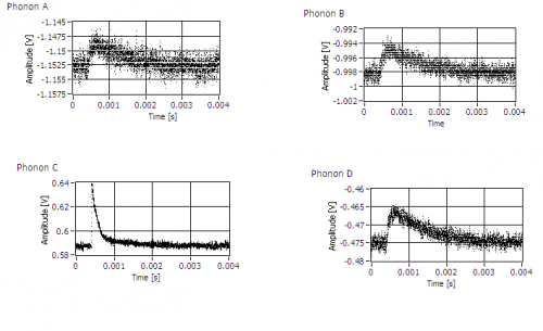
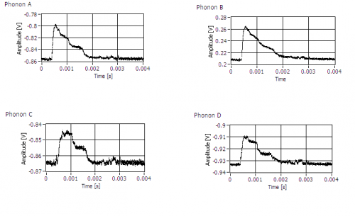
“Ugly” pulse shapes were pervasive this run. Some shapes appeared as though it could be good pulses with low-frequency noise on top, though many exhibited “shelving” as pictured below:

DIB1 (DCRC55) pulses with DIB2 (DCRC32) phonons in various conditions
DIB1→DCRC55 phonons
with DIB2 p-channels ON	with DIB2 p-channels OFF	with DIB2 turned off

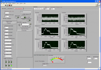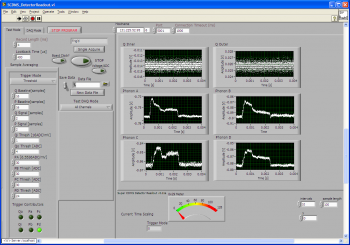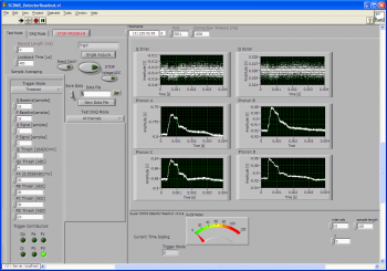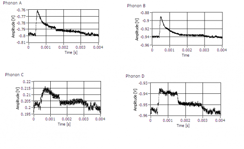
Showing that DIB1 (DCRC55) pulses are ugly regardless of DIB1 phonon settings. It was also seen that powering only one DCRC at a time helped the overall pulse shape:

Figure 1: DIB1 DCRC 55 pulses (no other DCRC connected)	Figure 2: DIB2 DCRC 33 pulses (no other DCRC connected)
Figure 3: DIB2 DCRC 33 pulses (no other DCRC connected)	Figure 4: DIB3 DCRC 50 pulses (no other DCRC connected)

The following is a first-pass attempt to calculate the total phonon collection efficiency for iZIPv6 G106a. This is defined as the total phonon energy measured in all 12 channels divided by the total phonon energy inferred from the calculated recoil energy of the event.

Our voltage-biased TES's are (to first approximation) kept at a fixed voltage and temperature by the feedback circuit. When phonons are absorbed by the TES the circuit reduces the current in order to compensate for the incident energy by decreasing the Joule heating. Knowing the voltage of the TES, we should be able to calculate the energy absorbed in an event by integrating the current pulse:

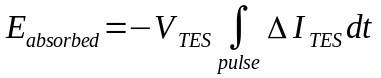
Among the QET settings is the QET bias current. Most of this current flows through the small 20 mΩ shunt resistor, so the the TES voltage is approximately the bias current times the shunt resistance.

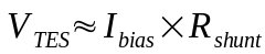
To integrate the pulse I use raw pulses, in ADC units per sample. The processing code produces pulse integrals as RQs, but I haven't been able to figure out the units or scaling. So for this study I use BatViewer to generate raw pulses in Root format from raw data. I use the first 100 samples to establish a baseline, then do a simple integral of the baseline-subtracted pulse (no filtering). One volt of output is represented by 2^14/2.5V = 6553.6 ADC units, and one sample represents 0.8 μs, so using these conversions I can express the integral in units of volt-seconds.

To convert from this raw voltage output to TES current we need to know the total gain:

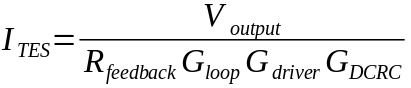
The feedback resistance is 1233 Ω and the SQUID loop gain is 10.5. The DCRC gain is a fixed value depending on the version: 5 for RevC, 2 for RevC.1. The driver gain, also known as “output gain”, is set by the operator, with values of 0-7 possible for RevC and values 1,2,4,8 possible for RevC.1. I got these numbers from Hassan who got them from conversations with Sten Hansen.

With the correct gain values this formula can be used to calculate the energy absorbed by one phonon channel. Summing over all channels gives the total phonon energy absorbed in the event. The total phonon energy produced by the event can be found if the recoil energy is known: it's the recoil energy times the Luke gain. So the phonon collection efficiency is

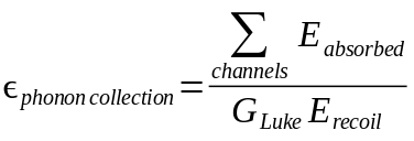
Assuming the event is an electron recoil the recoil energy can be determined from the charge calibration and the Luke gain is

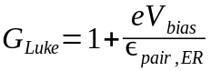
The bias voltage is the positive difference between the charge biases set for each side and the ER pair production energy is 3.0 eV. With a -4/+4 V bias the Luke gain is 3.67. For the recoil energy I use the calibrated Side 1 charge energy. Thus there is an implicit assumption that all events in consideration are electron recoils.

Using data from series 07150706_1856 (no external source, shield in place), I compared my integrated voltage quantities to the P*INTall RQs and determined an empirical conversion factor. This allowed me to use the processed RQs instead of raw pulses, which is much more convenient. Comparing several events I found that the adjusted RQs match my integrals within a few percent. I wouldn't expect them to agree exactly because CDMSbats uses filtering and probably a different range to find the baseline.

A few assumptions and approximations are used in the calculation of the absorbed energy above. For example we depend on knowledge of the QET bias current. This is selected by the user, but it is probably the case that it gets converted to a voltage by the LabVIEW vi or the DCRC by multiplying by the bias resistance. There could be errors then based on the calibration of the DCRC output or the true value of the bias resistance. The resistance of the stripline traces also introduces an error of a few 10ths of a percent. (Errors based on the TES and shunt resistances are much smaller.) Errors in the bias current will be neglected here, as they are in IbIs studies.

The approximate formula above for the TES voltage is only accurate to the extent that the shunt resistance is much smaller than the TES resistance. The shunt resistance is 20 mΩ while the resistance of the biased TES is usually around 200 mΩ and can in principle vary to as high as about 800 mΩ (the normal resistance) during a pulse. The TES voltage is thus significantly smaller than the estimate in the quiescent state, and also varies during the pulse. Below is a corrected version of the absorbed energy calculation (here is a derivation):

The parentheses represent the correction to the approximated absorbed energy calculation. The first correction term is fixed for a channel. It depends on the quiescent TES resistance in its biased state. Usually the bias current is chosen so that the quiescent TES resistance is about 200 mΩ. This means the first correction term is about -22%.

The second, non-linear correction term is a sort of average of the signal current during the pulse divided by the bias current. (Here “signal current” refers to the magnitude of the current deviation from the quiescent state.) To calculate this correction precisely would require a second pulse integral that is not available in the standard processed RQs. The size of the correction varies with the size of the pulse. The largest it could be would be for a completely saturated pulse; assuming 200 mΩ and 800 mΩ for the biased and normal TES resistances, the maximum is +7.5%. For events with smaller energies the correction will be much smaller. Using several events ranging from 60 keV to 800 keV I found that this correction can be estimated as (E_recoil / 1 MeV)*2.9%. Thus this correction is rather small for the energy range of interest.

The two corrections were applied to create a derived phonon collection efficiency quantity from the processed RQs.

The above treatment neglects any parasitic resistance. If there is a fixed parasitic resistance in series with the TES, the corrected energy equation is as follows:

The parasitic resistance referred to above is a fixed resistance in series with the TES. If there is another parasitic resistance in series with the shunt resistor, the shunt resistance can simply be considered as the sum of the shunt and its parasitic resistance.

Figure P1: Phonon collection efficiency for series 07150706_1856

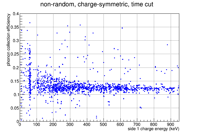The figure above shows the resulting calculated phonon collection efficiencies plotted versus calibrated Side 1 charge energy. Only a few cuts were applied: randoms removed, a charge symmetric selection, and also a time cut. The time cut selects the first ~half of this 15 minute series. After this time a bimodal behavior appears in the phonon quantities, manifesting in a double peak in the phonon energy spectrum and an extra band in the plot above, at low energies especially. Probably this is an intermittent noise effect that arises later in the run, distorting certain pulses.

At the 60 keV peak and for low energy events in general the efficiency is not very well defined, but it forms a tight band at higher energies. The mean is 12.4% for energies greater than 200 keV.

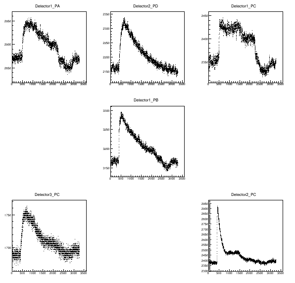
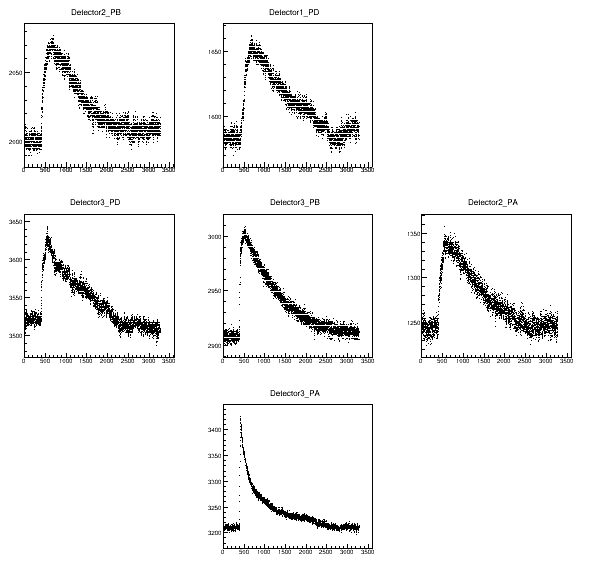
To get a clearer idea of how reliable the integrals are for this purpose, I show below pulses from a few representative events. The phonon pulses are arranged as they are on the crystal, with both sides arranged as viewed from above Side 1. (The outer ring channels are just inserted in a spare position: upper middle on Side 1, upper left on Side 2).

The pulses below are from a 60 keV event with approximately the “correct” efficiency (i.e. the efficiency seen in high energy events). There is significant distortion in many phonon channels.

Figure P2: 60 keV event with 17% phonon collection efficiency
Side 1	Side 2

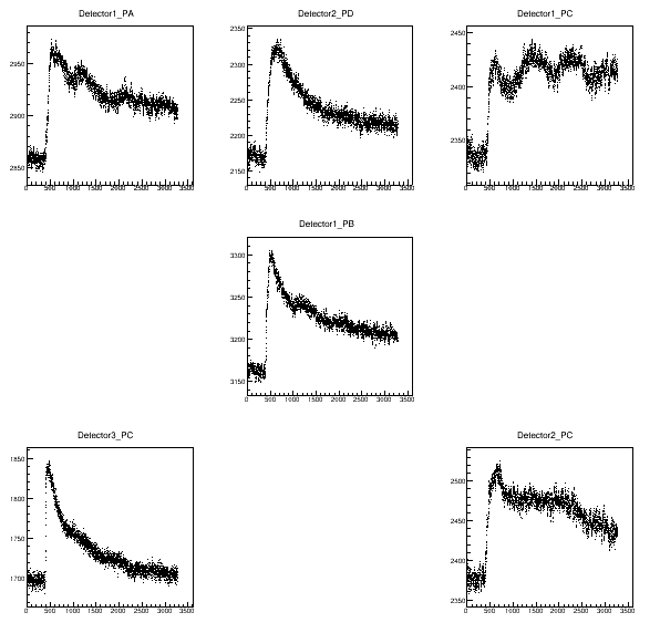
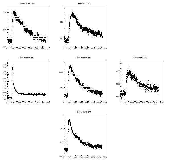
Below is a 60 keV event with a too-high efficiency. It seems to have been affected by a pulse distortion causing several channels to not relax to baseline, which is probably why the integrated amplitudes are too high.

Figure P3: 60 keV event with 26% phonon collection efficiency
Side 1	Side 2

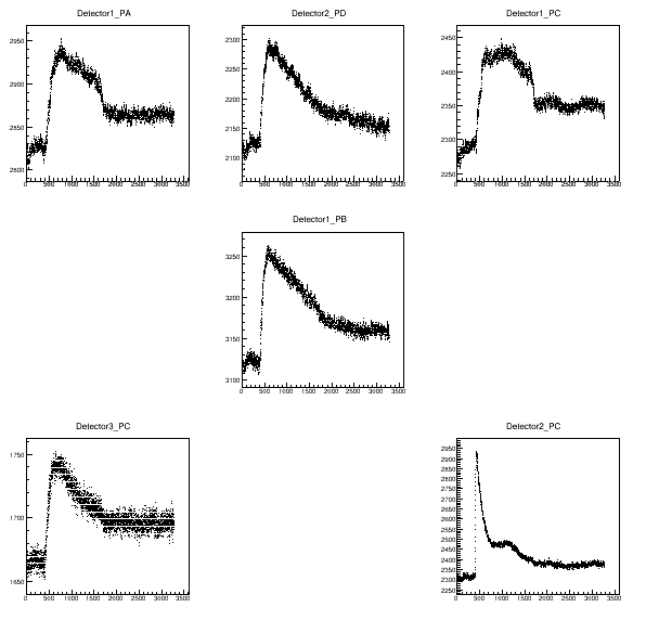
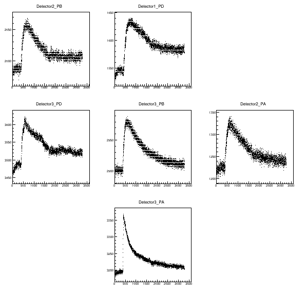
Below is another 60 keV event with too-high efficiency, this one during the later time period (in which a second, higher ~60 keV peak appears in the phonon energy spectrum). Here the “shelving” effect is evident. It's possible this particular sort of noise/distortion started showing up more frequently some time in the middle of the series.

Figure P4: 60 keV event with 28% phonon collection efficiency, late time
Side 1	Side 2

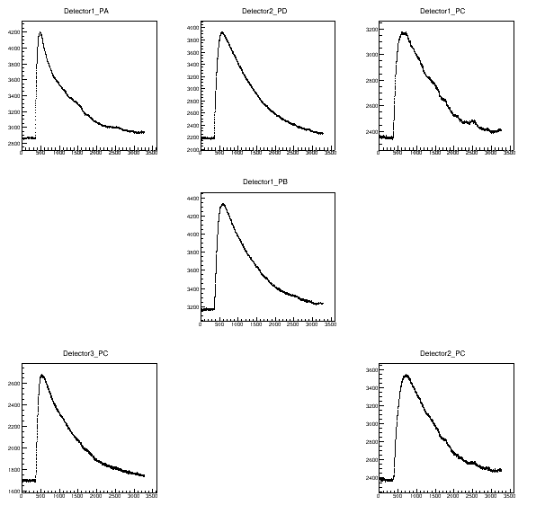
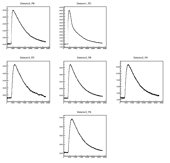
Below is a high-energy event with the correct efficiency. Noise is still evident in the pulses but it is small compared to signal.

Figure P5: 800 keV event with 15% phonon collection efficiency
Side 1	Side 2

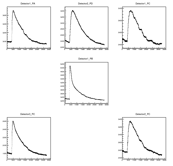
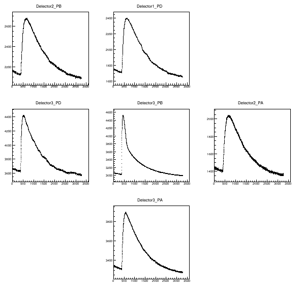
Below is a high-energy event that is an outlier in terms of phonon collection efficiency, only 11%. The downward slope of the pre-pulse suggests this event occurred on the tail of the preceding event. Probably this caused an overestimate of the baseline in the integration algorithm, causing the pulse areas to be underestimated.

Figure P6: 500 keV event with 11% phonon collection efficiency
Side 1	Side 2