Table of Contents
Run 65 Summary
This is a repeat of run 64 with shorted channels repaired.
Detector
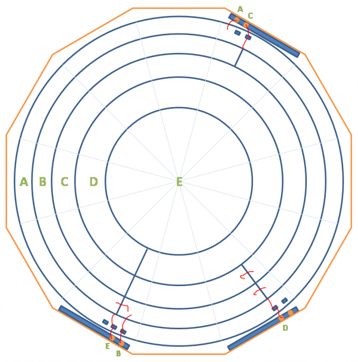 |
| Wirebonding plan for S1502 |
Wiring Plan for detector and switchboards
| DIB1qI | qA - outer |
|---|---|
| DIB4qI | qB |
| DIB1qO | qC |
| DIB3qO | qD |
| DIB4qO | qE -inner |
Contact free bias is run through DIB1 QETA + QETA ret lines. A pair of bias resistors in series on the DIB 1 switchboard allows for the leakage current to be measured, similar to the way it is done with the HV board.
- The large bias resistor is 10.95 MΩ
- Leakage measurement resistor is 1.03 kΩ
- This gives the formula for the bias at detector as: V_det = V_set - 1.06E4*V_leak
The voltage across the crystal is not the same as that applied to the detector as a whole because there is a voltage drop across the vacuum gap. By treating the gap and crystal as parallel plate capacitors in series, one obtains.
- V_crystal = V_det/(1+ε_Si/ε_0 * d_gap/d_Si)
- ε_Si/ε_0=11.68 (Wikipedia), d_gap=0.037“±0.004” (2017/09/08), and d_Si=1“
- V_crystal = V_det*(0.70±0.03)
LEDs
- Two IR and two UV LEDs are mounted on the electrode. These are connected to phonon leads on DIB3
- To operate these, the DIB3 switchboard must have DIP switches 1,2 on switch package 6 turned off to disconnect the DIB LEDs. These are located on the underside of the board.
- Additionally, the 4 switches on the red DIP switch package must be turned on. These connect the electrode LEDs to the DCRC.
- With the switches set as above, the electrode IR LEDs can be operated on DIB3 with a positive LED bias current while the UV electrode LEDs will run with a negative bias current.
- Four functioning IR LEDs are mounted on the detector DIBs, on DIB3 and DIB4, situated on the charge channel side (opposite the external electrode)
- To operate these LEDs the DIB3 switchboard must have DIP switches 1,2 on package 6 turned on and the the 4 switches on the red DIP switch package must be turned off. This will connect the DIB3 DIB LEDs. The DIB4 LEDs are also always connected.
Cross Talk
Charge Collection Efficiency
Extracting carrier lifetimes from CCE (turned out to be a bad model, see “CCE model” below)
Peak Shoulders
Update: See CCE analysis above. This may have just been an artifact of bias in the OF fits.
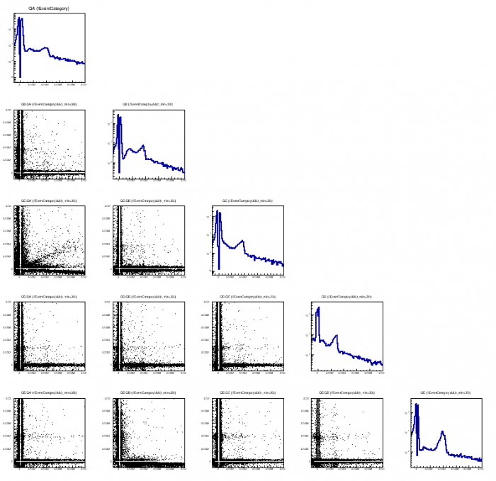 |
| The above shows the same plots for the 70V data series 07171023_1041. This data set had better tuned trigger levels and avoided spurious noise triggering. The scale is also 2 orders of magnitude smaller than the previous plot. |
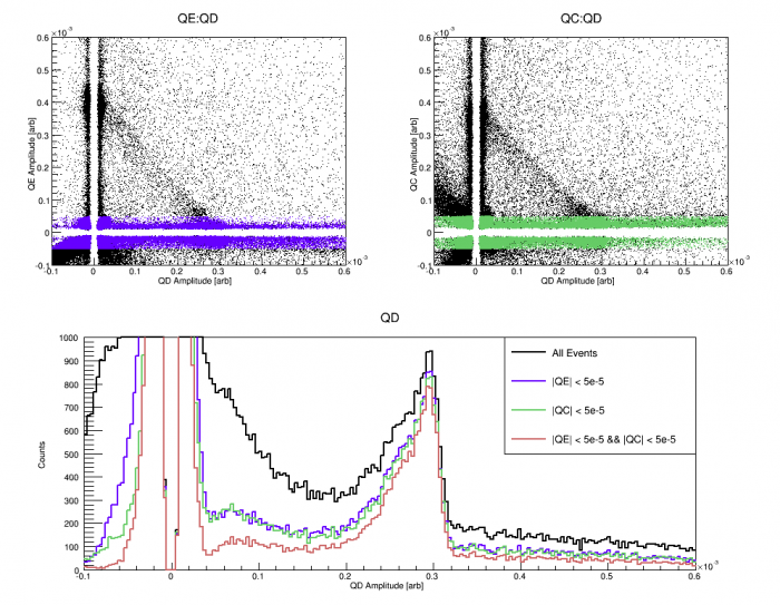 |
| This is an example of signal sharing between QD and the adjacent channels in 90V data (07171023_1618). The 60 keV events can be seen as a diagonal line in the first two plots. These are events for which the signal is shared. The lower plot shows that cutting out shared events still does not produce a gaussian distributions in a single channel. |
Hold Time
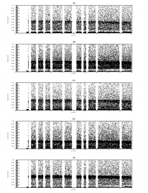 |
| Channel amplitudes vs time in 70V data (07171023_1041) |
const
Neutralization Loss
After a certain amount of time running under bias, the charge collection efficiency falls off dramatically. This can be tracked by plotting the 60 keV peak position versus time. Data at a variety of biases was examined - in each case the bias was applied to the external electrode with the detector charge channels grounded. The points at which the peak amplitude fell to 90%, 80%, and 60% were determined by eye. The 80% and 90% points were extrapolated back to 100% to define a “hold time”.
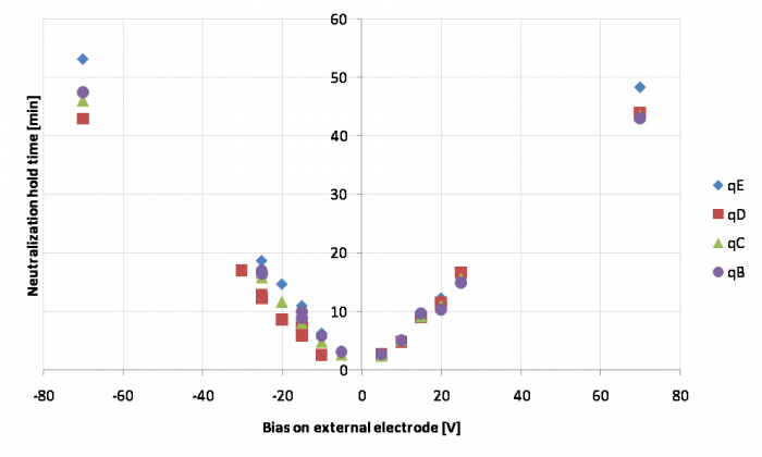 | 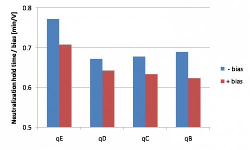 |
| The left plot shows hold time versus applied bias. There is a fairly well-defined slope in each case. These are shown in the right plot, which indicates some variation in hold time with respect to bias polarity and channel. |
|
A couple of mechanisms can produce the drop in charge collection efficiency from neutralization loss. One model for this run is that the loss is dominated by surface charge building up on the detector, since one side has a vacuum interface. As ionizing events produce charges, they drift to the vacuum side and are stuck there. This would produce a buildup of surface charge at a fixed rate. As the surface charge builds up a counter-field is produced, so that the effective bias on the detector decreases. As seen in the seagull plots, a low bias will decrease the charge collection efficiency.
This model fits the observation above the negative biases produce longer hold times than positive biases. We expect the effective bias to fall at the same rate in either case, but as is seen in the seagull plots, a low bias has a stronger effect on charge collection efficiency in the case of positive biases - hence shorter hold times for positive biases.
By combining the hold time data (specifically the 80% and 60% points) with the seagull plot data, we can estimate what the counter-bias is as a function of time. To do so I fit the individual seagull curves for each channel and each polarity to a (empirical) power law. Below is a plot of counter-bias versus time using data taken at the different biases.
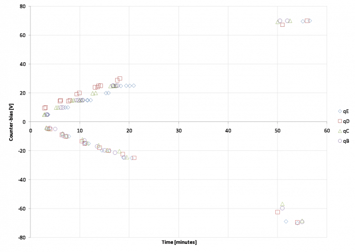 | 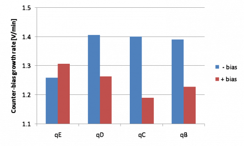 |
| Counter-bias versus time. For most of the channels this is quite linear, which supports the model that the drop in charge collection efficiency is mostly due to accumulating surface charge from ionizing events. The rate at which effective counter bias grows is shown on the right for each channel and polarity; there is some variation. |
|
From this model of neutralization loss the bias on the detector should be

where h is the detector thickness, d is the gap between detector and electrode, κ is the dielectric constant of the detector (11.45 for Si near 0K), and σ is the surface charge density. This ignores any fringing and assumes uniform charge density. At σ=0 (when the bias is first applied) the detector bias is smaller than the electrode bias by a factor of 68% (h=1”, d=0.037“).
The second term in parenthesis is the so-called counter-bias, the effective reduction in applied bias. Using the rates found for increasing counter-bias, we can calculated the growth rate of σ. Assuming this is due to ionizing events, we can calculate the rate of energy deposition (using 3.8 eV / charge pair for Si), which should be the product of the event rate and the mean event energy. Using a radius of 75 mm and the observed counter-bias growth rate of 1.25 V/min, this implies an energy deposition rate from ionizing events of 82.1 MeV/s.
What is the apparent rate of energy deposition based on the observed spectrum? I calculated the raw event rate by counting the number of random traces with visible pulses in any of the channels, using one set of data (40 V data from 2017 October 24) and found 165 Hz. This is quite high, a consequence of using 4 Am sources and no shield apparently. Then I attempted to find the average energy per event. This can be calculated directly from a full-range spectrum, if the energy calibration is reliable over the full range. I selected data before neutralization loss (first 20 minutes), calibrated each channel to 60 keV, then created a summed energy quantity that adds all channels that are above 10 keV. (Without this threshold there tends to be smearing from under-fit pulseless traces in neighboring channels.) I found the average energy per event to be 558 keV. This yields an energy deposition rate of 92.2 MeV/s, approximately in agreement with the rate implied by the growth rate of surface charge.
UPDATE: I refined the calculation of the average energy per event. First, I readjusted the total charge calibration to recenter the 60keV peak (about a 1% correction). Second, I tried to account for below-threshold events. I assumed that events below threshold have a flat spectrum down to 0 keV, and used the spectrum just above the noise wall to estimate the height of the low-energy spectrum. The adjusted average energy per event is lower, 547 keV. This yields a somewhat lower energy deposition rate of 90.3 MeV/s, closer to the rate implied by the surface charge.
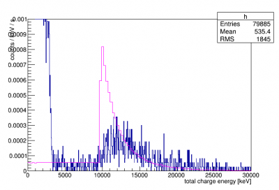
Below are plots of the spectrum in three energy ranges:
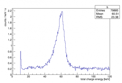 | 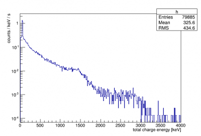 | 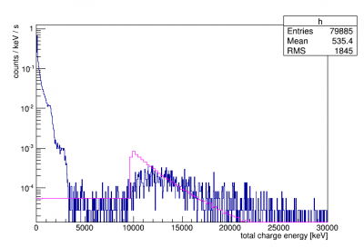 |
| 60 keV peak is reasonably well calibrated but smears to lower energies | Here there are hints of the 2.6 MeV (highest U/Th line) and maybe the 1.4 MeV K line | Here a simulated muon spectrum is superimposed |
 |
UPDATE:We are trying to refine the calculation of energy deposition rate from inferred counter bias. The calculation above assumes the the surface charge accumulates at a constant rate equal to that of the energy deposition rate from ionizing events in the crystal. However, as the CCE decreases, less of each event's carriers will make it to the electrodes without recombining/capturing. This means that the rate of surface charge accumulation will decrease with the CCE. This means the above calculations should underestimate the true rate of energy deposition from ionizing events. A Google doc model of this effect has been made here. It assumes a constant energy ionizing energy deposition rate and the CCE to calculate the rate of surface charge accumulation a one time step. Then it finds the total amount of accumulated charge, the resulting counter bias, and the effective bias in the detector. It then uses this to update the CCE (using power law parameterizations of seagull plots) for the next time step and repeats.
The figures below show an example of the generated counter bias and signal as a function of time. The plot on the left demonstrates the difference in counter bias if the charge accumulation rate is assumed constant (blue) and when the changing CCE is accounted for (red). The difference is small, but can change the inferred true event rate by 5-10%. An example of the resulting 60keV signal as a function of time is shown on the right. It qualitatively matches those observed in data. Below CCE~0.6, the CCE parameterizations fall off quickly and are no longer valid. This occurs when the counter bias is nearly the same as the total bias.
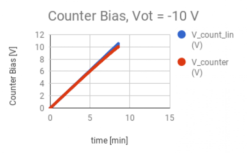 | 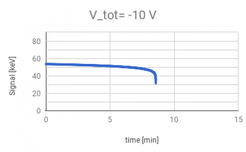 |
Using this model, the signals were modeled over the range of Vtot biases used in data ( -110V to 110 V) using 90.3 MeV/s as the true event rate. This is the rate calculated above from the energy spectrum. The average CCE fit parameters for positive and negative biases were used. In each case, the constant rate one would infer given the fall times is also calculated. The figure below shows these inferred constant linear rates as a function of bias. Also shown are the true rate used (90.3 MeV/s) and the measured constant rate from above (82.1 MeV/s).
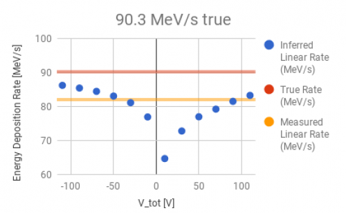 |
At most biases, the modeled, inferred linear rate is consistent with the measured value. This shows that the true energy deposition rate calculated from measured spectra is consistent with the observed signal fall times.
An easier way to see the agreement is to compare the measured 60% and 80% hold times to those calculated by the model. This is shown in the figures below. The measured values here are taken directly from the data; they are the times at which the peak has fallen to 80% and 60% of its starting value at the beginning of data taking. As described above, the model assumes a true 90.3 MeV/s event rate, but accounts for the changing CCE as a counter bias develops. The model uses the average CCE curve of the positive and negative bias data and the uncertainty comes from the spread in individual channels' CCE curves. Although some of the values don't match at low Vtot, there is a remarkably good agreement overall.
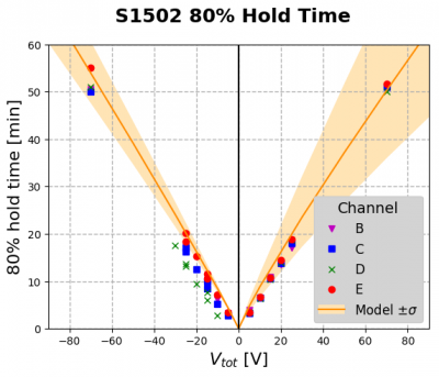 | 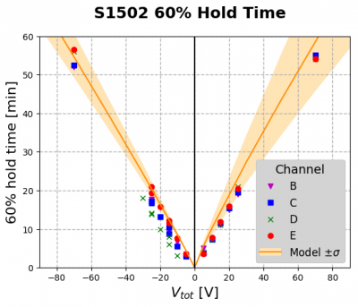 |
Additionally, here is a plot illustrating more clearly the behavior of the model. It shows how the accumulating counter bias causes the observed signal to decrease as a result of the reduced CCE. The dashed line shows the initial counter bias slope and illustrates how the slope changes over time.
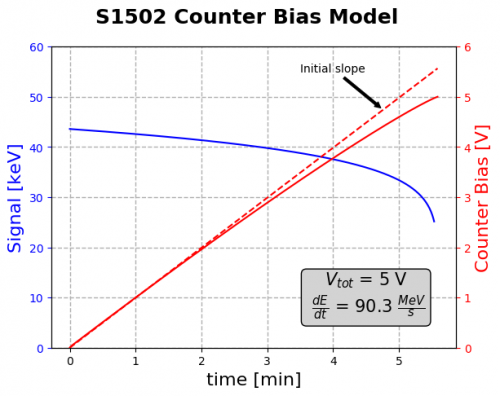 |
old version:  had an error. Old text: Calibrated spectra suggest a mean deposited energy around 300 keV per event. Combining this with a counter-bias growth rate around 1.25 V/min yields an event rate around 25 Hz. This is a plausible event rate, which lends credence to the model.
Re-neutralization and LED performance
We tested neutralization using different amounts of flashing from the different LEDs (IR mounted on electrode or on DIBs, UV mounted on electrode) while the detector was grounded. The most dramatic observation was that we could reduce the amount of flashing by 4 orders of magnitude and still neutralize just as effectively.
The tests were done with a 10 V bias, which with a standard flash provides 7 minutes of hold time. We considered this full neutralization.
We modified the following:
- which LEDs were used
- total flash time
- time between individual LED pulses
- LED pulse width
Another important observation was that grounding with no flashing at all also neutralized the detector. Grounding for 5 minutes (which is close to the standard wait time after flashing) produced partial neutralization (4 minute hold time); grounding for 25 minutes produces full neutralization.
With a 5-minute wait time we compared the different kinds of LEDs with different amounts of flashing:
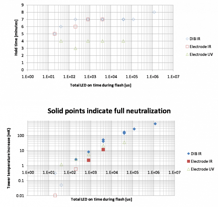
The upper plot indicates that the IR LEDs on both the electrode and the DIB provided full neutralization over a wide range of total on-times. The DIB ones performed a little better, providing full neutralization at lower on-times. The UV LEDs however did not neutralize any better than no flashing at all.
The lower plot shows that for the IR LEDs the temperature increase of the tower was a good predictor of whether the detector neutralized completely. But the UV LEDs, although they seemed to be dumping the same amount of power, did not help neutralize the detector.
There is a data table on the run diary.
Another test performed was to take data at 50 V until losing neutralization, then ground the detector and continue to take data. We found as we had expected that the detector provided its own bias due to the leftover surface charge density, and we were able to see full energy events without any external bias:
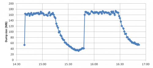 |
| Initial hold time = 35 minutes; hold time after removing bias = 40 minutes |
The “self-biased” hold time was nearly the same as the externally-biased hold time, which makes sense considering the mechanism of neutralization loss described above.
Simulation
A simple simulation of the R65 crystal with Am sources was performed in Geant. The simulation consisted of a 6” diameter, 1“ thick Si cylinder with 4 59.54 keV sources positioned at the appropriate radii. Unlike the real detector, the simulated sources are all located at the same angle on the detector for ease of analysis.
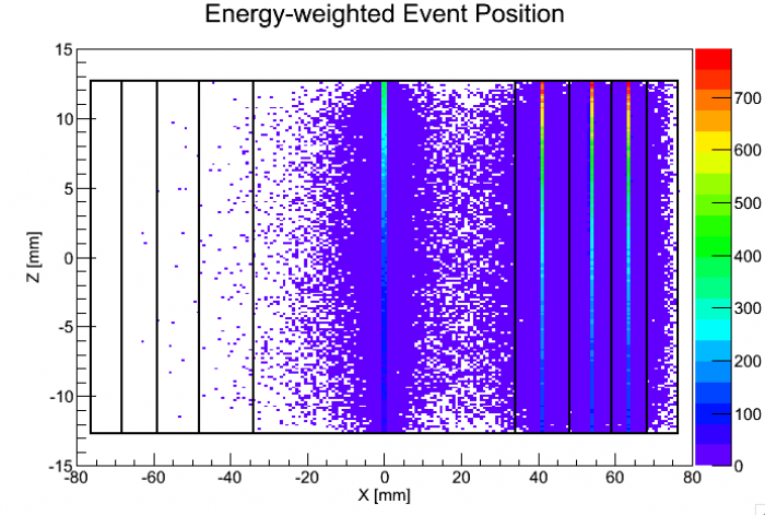 |
| The above plot shows the energy-weighted position of 60keV events in the detector. The detector and channel boundaries are shown for reference. While the events seem mostly localized in a column beneath each channel, there are certainly some stray events at high radius. |
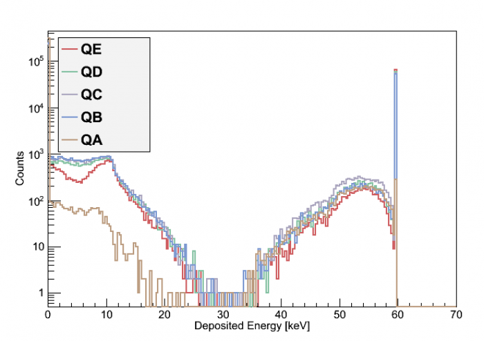 |
| For the above plot, the energy deposited beneath each channel was determined for each gamma thrown. This demonstrates that only ~1% of the 60keV smearing is directly due to spread of initial deposited energy. To calculated the signal seen by each channel, the charge propagation across Ramo potentials must also be considered. |
Comparing Am Rates
Looking at 60 KeV event rates over each channel for different biases and comparing the ratio of each channel to qD.
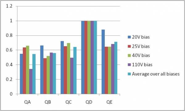 |
| Above plot shows positive biases of all channels, including average over all biases. |
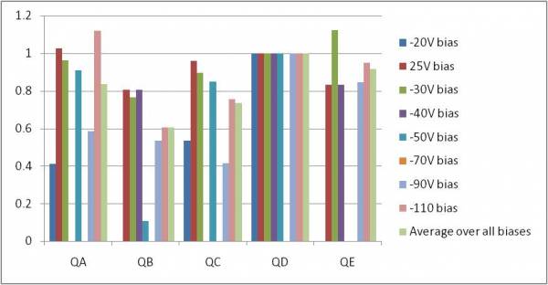 |
| Above plot shows negative biases of all channels, including average over all biases. -70V bias data was weird over all channels, will have to look closer at the sequence. |