Table of Contents
Charge Collection Efficiency
The 60keV signal amplitude as a function of bias voltage and radius was studied to investigate charge collection efficiency. There are believed to be several mechanisms which affect charge signal amplitude including impurity trapping, counter fields, and drift time.
A few basic cuts were used for this analysis.
- Randoms removed
- Channel being fit is the largest for that event
- Time cut to ensure peak has not shifted since series began
The 60keV peak in channel E appeared to be gaussian, but those in A-D were not. They all seemed to be smeared to low energy, with more such smearing at high radius. For this analysis, channel E's full peak was fit with a gaussian, while only the high-energy side of the 60keV peak was fit in channels A-D. All fits were performed with a linear background in the peak neighborhood.
| Figure 1 | ||
|---|---|---|
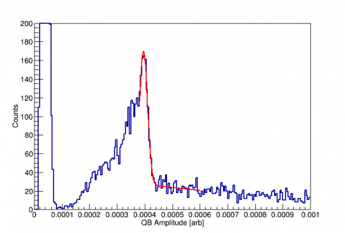 | 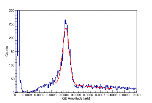 | |
| The above show examples of fitting an outer channel (left) and central channel (right). | ||
First Pass
| Figure 2 |
|---|
 |
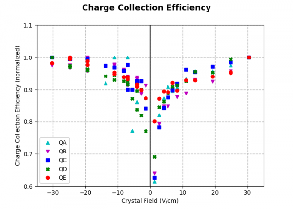 |
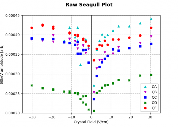
| The first plot shows the channel amplitudes as a function of field applied to the crystal. The polarity is relative to the contact-free electrode. Channel D was read out with a revC DCRC which has a lower driver gain. The second plot shows the same data with each channel normalized to its maximum value for that bias polarity. All channels are reaching 90% charge collection efficiency by ~ 8 V/cm. Note: Currently the 60keV peak is absent in much of the QA data taken with negative biases. cce_data.xls |
Absolute Calibration
Historically these “seagull plots” have been given relative normalizations with 100% charge collection efficiency being defined as the maximum achieved, which is usually where the plot flattens out. However, it should be possible to calculate the absolute gains in the charge measurement channels and obtain an absolute calibration. The conversion from output voltage back to actual amount of charge induced on the electrode depends on both the intrinsic DCRC gains and the conversion from measured charge to voltage at the first amplifier stage. As described in many CDMS theses (e.g. Phipps, Golwala) The voltage measured is (to 0th order) the charge seen by the first amplifier stage over the stray capacitance of the feedback network.
Vout = Qsig/Cfb
Since the feedback resistor is known, this capacitance can be obtained by fitting the pulse fall times. For Run65, the average fall time was 46.2 us, making this average capacitance 1.15 pF. As discussed at the end of this run's crosstalk analysis, there are further corrections that depend on the coupling capacitor and other capacitances present at the measurement electrode. This combination of capacitances gives an effective gain of
Gcap = C_coupling/(C_coupling+C_ground+C_otherChannels) = 0.81 ± 0.04
After that, the DCRC has a few stages of further amplification and filtering before the voltage is digitized. These gains are different depending on the DCRC rev. To determine these gains experimentally, we used a miniBob to feed a square wave signal into the charge channels. Then, we used an oscilloscope to measure the pulse height at test point 5, the output of the first amplifier stage. We found that the Rev C and C.1 boards operated identically this far. Then, we compared these pulse heights as recorded by MIDAS in data. This showed that the built-in gains for our boards are
| Charge Channel Gain | |
|---|---|
| Rev C | 4 |
| Rev C.1 | 5.5 |
This ratio has been confirmed numerous times in our data, but now we also have the absolute gains. Putting these pieces together allows us to calibrate from the RQ 'OFnoXvolts' back to charge induced at the electrode. This calibration was then used to generate absolute charge collection efficiency for this detector. The results of these corrections are shown in figure 3 below. Also shown for reference is the CCE plot from run 60, the single channel bare 150mm device (S1501). Note that the S1501 data has the highest CCE defined as 1.
| Figure 3 | |
|---|---|
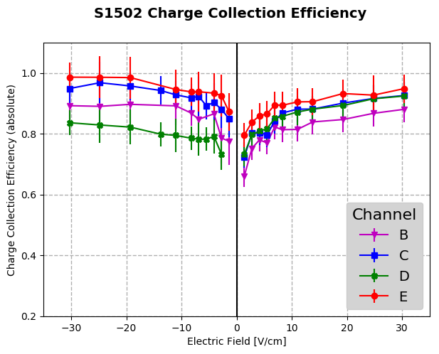 | 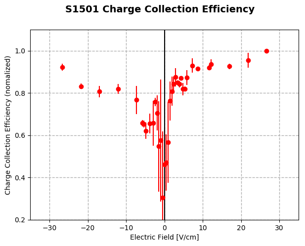 |
Both devices show an overall asymmetry with sign of bias. It is important to note that the calibration sources were on opposite electrodes for the two devices; they were on the readout electrode side for S1501 and the bias electrode for S1502. This means that, for events occurring near the source location in S1501, the majority of the signal was from electrons for positive biases and holes for negative. It is the reverse for S1502. So it seems that, in both devices, electrons generally had higher charge collection efficiency than holes for a given field magnitude.
However, there is a possible additional wrinkle. All data shown here was taken with QD on a RevC dcrc while the other channels used rev C.1 boards. One difference in the boards is the overall sign of the gains. i.e. The recorded pulses for QD were always opposite in sign to those on the other channels. For positive biases, as labeled in the run65 seagull plot above, the Rev C.1 boards give negative pulses while the rev C board gives positive pulses. Asymmetry in charge signals with bias polarity has been observed before but the source has not been understood. It is suspicious that this seagull plot shows larger CCE (larger signal) for the bias with positive-going pulses, regardless of DCRC board. The run60 data was taken with a rev C.1 board, so positive biases correspond to negative pulses. However, in this data, the negative pulses are stronger.
A quick look at the processed data shows that the ratio of OF amplitudes (specifically QEOFnoXvolts) to pulse height (QEmax) is independent of the bias voltage. However, the max quantity has been filtered, and may not be a reliable measure of the absolute pulse height.
While trying to measure the absolute DCRC gains, data was recoded with each dcrc's charge channel driven by a square wave via the miniBob. A search for peak asymmetries in these data sets (07180117_1513 and 07180117_1520) showed no difference in positive/negative pulse amplitudes greater than 0.5% for either dcrc version. positve/negative (RevC) = 1.004, positve/negative (RevC.1) = 0.9976. However, this warm bench test may not be a faithful reproduction of the circuit operation with cold electronics. These tests were done with a relatively large input signal. Later tests (below) found more substantial asymmetry at signal sizes near that of 60keV events.
It could be that there are two effects here. The first is that the RevC board shows this asymmetry, with positive (negative) pulses being too high (low). This would bring the run 65 data into a little more order. The second is that there is also a difference in electron and hole trapping in these crystals, with electrons having less trapping and higher CCE.
OF Amplitude Glitch
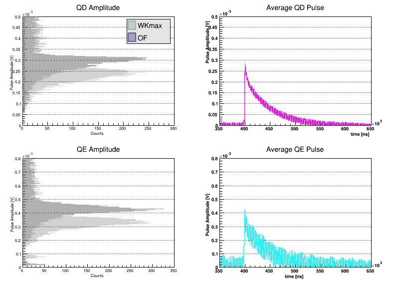
Comparing the fit amplitudes to the actual traces indicates that the OF is currently returning amplitudes that are somewhat higher than expected. Example fits of two events are shown in figure 4. The template is overlayed with both the OF amplitude and the WKmax amplitude. The WKmax is simply the maximum height of the pulse after a 2nd order Butterworth filter has been applied.
| Figure 4 | |
|---|---|
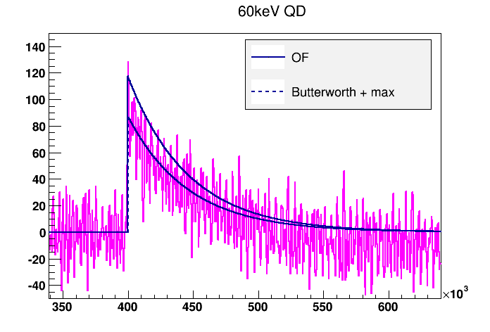 | 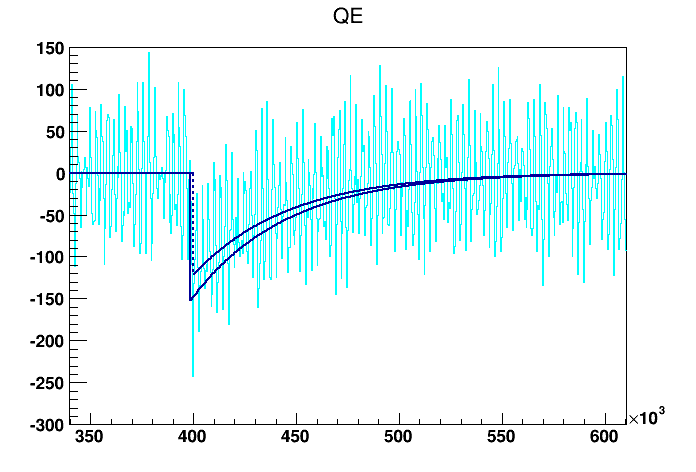 |
It seems clear that the OF is returning too high of an amplitude while the WKmax quantity is doing a better job. This can be seen en-masse in figure 5. There the distribution of fit amplitudes are shown on the left along with the average pulse on the right. The top row is for QD on a revC and the bottom for QE on a rev C.1. The distributions and average pulses are constructed from ~1000 events. The two amplitude estimators are clearly in tension with each other, with the WKmax quantity about 80% as large as the OF. If the max quantity is correct, this will shift the CCE seagull plots by that same factor.
| Figure 5 |
|---|
 |
At this point it is unknown why the OF seems to be failing. We have tried modifying the template rise time and making the cut for noise events used in generating the optimal filter more strict. Neither has had a noticeable effect.
WKmax CCE and Improved Signal Estimation
The charge collection efficiency seagull plot was recalculated using the WKmax quantity described above. Cuts on 20% rise time and to ensure that the channel being fit was the maximum channel were used. It appeared that the distributions were much more gaussian using this quantity. The one-sidedness described above was greatly reduced in all channels. This may have been an OF fitting artifact due to the OF preferring high amplitudes. This seagull plot is shown below in figure 6. The measured signal is in units of charge measured at the channel electrode in atto-Coulomb. This is because we are fairly certain of the calibration up to that point.
| Figure 6 |
|---|
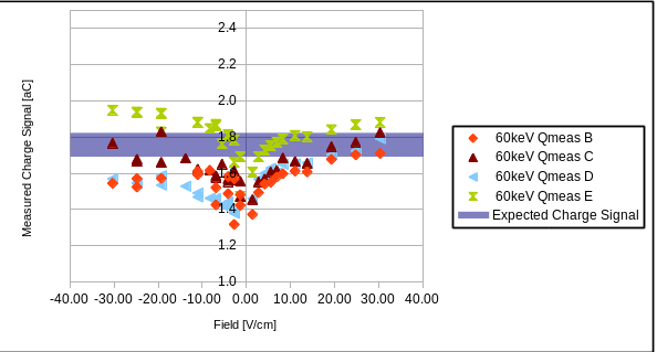 |
Additionally, progress has been made on understanding the expected signal. In particular, it was realized that, due to the vacuum gap, the charges never traverse the entire Ramo potential, which means that we expect a reduced amount of charge at the electrode. It further turns out that one must consider the different dielectric materials in the detector bulk when calculating the Ramo potential. The result is that the measured signal is expected to be reduced by the factor h/(h+kd) = 0.70 ± 0.03 where h is the crystal width, d is the gap width, and k is the Si dielectric constant. This expected signal is also shown on the plot.
OF amplitude repaired
After a bit of digging, it was eventually discovered that there was an error in the portion of the cdmsbats code responsible for loading normalizations for the OF calculation. In particular, the following lines in “BatRoot/EventBuilder.cxx”. These create an OptimalFilterNxN object to do the calculations and then give it some templates and normalizations. The LoadTemplates and LoadNormalizations functions use the trace sample time in normalizing the optimalfilter. As the code was, the sample time wasn't set until later and the default sample time (0.8us) was used as opposed to the correct value of 0.4us for charge channels. This has been fixed by simply loading the sample time before the normalizations.
// ---------- Instantiate and load parameters ---------

OptimalFilterNxN myOptimalFilterCharge("OptimalFilterCharge");
myOptimalFilterCharge.LoadTemplates(templateFFT, templateConjNoiseFFT,chanName);
myOptimalFilterCharge.LoadNormalizations(sigToNoiseSq, noiseFFTsq, templateMax, chanName);


//set timing parameters
myOptimalFilterCharge.SetSampleTime(1.0/sampleRate);
myOptimalFilterCharge.SetXwindows(qxwinMin, qxwinMax,traceLength);
This bug resulted in the OF amplitudes being too high by a factor of sqrt(2). This means that the amplitudes calculated before can still be used, but with this correction. i.e. the OF-based seagull plot in figure 3 has the correct shape, not needs to be renormalized for this sqrt(2) effect (and to account for the reduced Ramo signal). Strangely enough, these two effects almost perfectly offset and rescale CCE in figure 3 by a factor of 1.0101.
Final Results
After the above Optimal Filter Amplitude issue was discovered, it was a simple matter to apply a correction of 1/sqrt(2) to the existing OF fit data. This, along with the reduced expected signal due to Ramo potentials, takes us back to the following seagull plot (reproduced from figure 3).
| Figure 7 |
|---|
| |
Now we can tackle the asymmetries observed. The asymmetry of the seagull plot corresponds to upright/inverted pulses for both DCRCs. We can try to quantify this ratio by looking at the ratios of upright/inverted 60keV amplitudes at the same total bias for each channel. i.e. Calculate the ratio of the QE (RevC.1) peak at -50V to that at 50V and compare it to the ratio of QD's (RevC) 50V peak over it's -50V peak. This is shown in figure 8.
| Figure 8 |
|---|
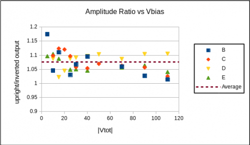 |
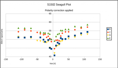
Note that QD is a revC dcrc while the others are revC.1. This makes it clear that there is a single ratio by which upright pulses in either DCRC are larger than inverted ones, that is invariant of bias voltage polarity. In general, upright pulses are 7.6±1.0 % larger than inverted pulses. This agrees with Matt's earlier findings of a ~5% reduction in inverted pulses. These same effects have not been observed when inputting signals directly into DCRCs on the bench( Data taken on 2018/02/07). It is believed that they are dependent on the cold electronics, perhaps the way the FET itself is operated. At any rate, the above plot indicates that it is a constant value which we can then correct for. Because we don't know which polarity is the “correct” one, we rescale both to the average, using the average ratio calculated above. This gives us a more symmetric seagull plot as shown in figure 9.
| Figure 9 |
|---|
 |
Next, we include DCRC-dependent corrections. In particular, second order corrections to the measured DCRC gains of 4 and 5.5 for the rev C and C.1 respectively. Because these gain stages are in the DCRC, they can be measured on the bench. As described here, a signal generator and minibob were used to feed a constant signal into each DCRC. The ratio of the output pulse amplitudes for the same input pulse polarity were then calculated. It was found that, for both polarities of input signal, the revC.1 output an pulse which was 12.9±0.6 % larger than the revC. Again, we don't know which is the “correct” set of absolute gains, so we scale both to the average value. This gives us the seagull plot shown in figure 10.
| Figure 10 |
|---|
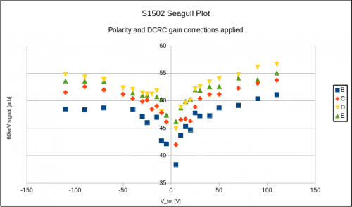 |
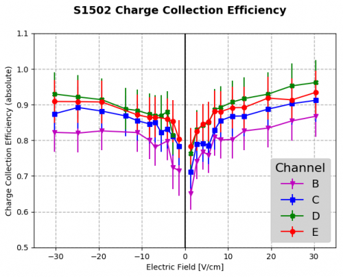
Now we can finally start to see some sensible structure. The inner channels, E and D, seem to have better collection while C and certainly B are lower. Putting in all the factors and uncertainties to scale this arbitrary signal to absolute CCE (e.g. sqrt(2) factor form cdmsbats error, Ramo reduction factor) and calculating the field in the detector gives us the final plot, figure 11. Here it is not only clear that the inner channels have better charge collection at a given bias, but that the CCE is approaching 100% in an absolute sense. There still may be some electron/hole asymmetry, perhaps favoring hole collection. However the effect is small, and is within uncertainties.
The pulse polarity correction factor can also be made to normalize the run 60 data. As shown below, this also gives a much more symmetric seagull plot, which provides further support for the appropriateness of this factor.
| Figure 11 | |
|---|---|
 |  |
Systematic Uncertainties
Most of the uncertainty in CCE values is systematic, coming from the absolute calibration, expected signal size, and gain corrections. These contribute to the generally large error bars in figure 11. The uncertainty of fit peak positions is actually quite small. These two effects can be more clearly separated by using the error bars to demonstrate fit uncertainties, and a band to show the overall systematic uncertainty on the CCE scale. This is shown in figure 12.
| Figure 12 |
|---|
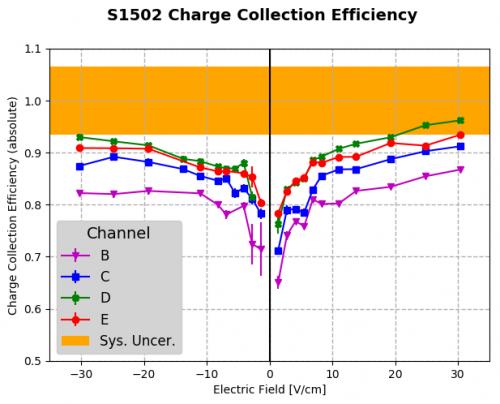 |
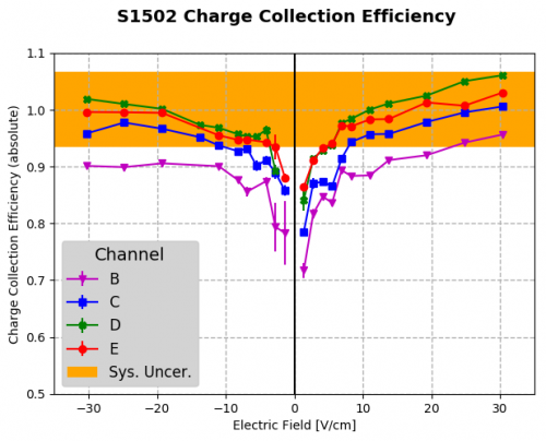
As described in the section above, one must choose which DCRC and polarity to use as the “correct” standard. For figure 12, this choice was avoided and the average was used. The systematic uncertainties represented include the uncertainty of the correction factors used. If instead of using the averages, one uses the observation that inverted pulses appear distorted and that upright pulses with the more advanced board (C.1) should be used as the standard, a more optimistic result is obtained. This is demonstrated in figure 13. Here, upright pulses on the RevC.1 board have been used as the benchmark, with the others scaled using the correction factors described above.
| Figure 13 |
|---|
 |
CCE vs Radius
The CCE plots above seem to show a trend for decreasing CCE with increasing radius. This is demonstrated in figure 14. Here, at each bias voltage, the CCE's have been normalized to the largest value and then plotted as a function of the calibration source radial positions. The innermost channel, E is at radius 0.
| Figure 14 |
|---|
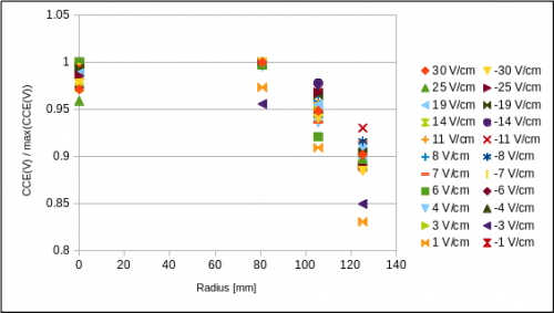 |
As is, the calculations assume a Ramo potential which is constant in radius. We are assuming that a 60keV event under channel E will induce the same amount of charge on E's electrode as a 60keV event under channel B will induce in B's electrode. However, we expect that the bias and Ramo fields change at large radii as fringing fields and the grounded housing start to matter. To understand these effects, it is necessary to model the bias field, Ramo potential, and charge motion in the field.