Charge Collection Efficiency Model
We would like to develop a model to explain the charge collection efficiency. Some combination of trapping and carrier recombination causes the signal to degrade at low bias field.
Penn et al. (1996) did a bunch of measurements of CCE on Si samples of various thickness and impurity levels. The takeaway is that, for high purity crystals, like the one S1502 is made from, there is very little “simple” trapping as the charges drift across the crystal. It assumes a field dependent average trapping length. Most of the loss seems to be in the initial charge cloud. For less pure crystals, it seems to be a combination of losses in the initial cloud and as the charges drift. This was inferred by considering how the simple trapping model should cause CCE to scale for detectors of various thickness.
Simple Trapping
The simple trapping model assumes carriers only trap while drifting with a field dependent average trapping length of the form
<m>\lambda=cE^m</m>
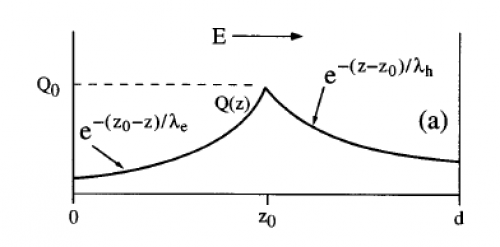
It turns out that only the average trapping length <m>\lambda = 1/2 (\lambda_e + \lambda_h)</m> matters. A diagram of the model is shown in Fig. 1 below. The population of each carrier type falls exponentially with distance from the event.
| Figure 1 |
|---|
 |
Penn's 15kΩ-cm samples are the closest to our current impurity level. Figure 2 shows Penn's and our measured CCE as a function of bias field. The Penn data does not show variation with detector thickness from 2.24 mm to 4.8 mm thick. A fit of the “simple” trapping while drifting model to the 2.24 mm data is shown as a dashed green line. If this is the correct trapping model, it should scale based on the detector thickness. Scaling that fit to 4.8 mm and 25.4 mm thicknesses are shown as dotted and dashed lines. It's clear, even from the Penn data, that this is not a viable model.
| Figure 2 |
|---|
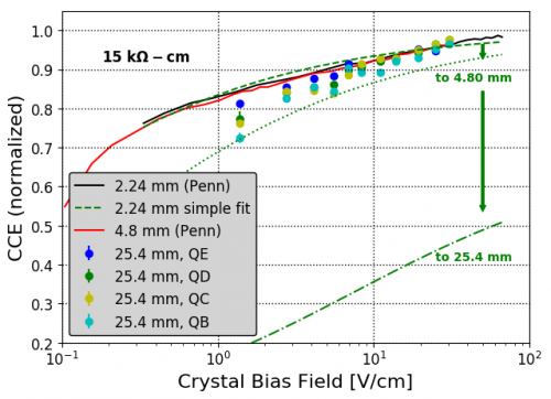 |
Our measured S1502 data does start to show some CCE loss at low bias fields, though not enough to be explained by the simple trapping model. It is therefor dominated by loss in the initial charge cloud.
Hybrid Trapping
Penn et al. developed a hybrid model which includes a crude model of charge lost in the initial charge cloud as well as any drifting losses thereafter. It assumes the initial cloud of charges shields itself from the applied bias field and that trapping occurs as the carriers diffuse in the field-free region within. If they diffuse with a mean free path, or constant “step length”, <m>\lambda_{step}</m> and have a constant trapping length, <m>\lambda_{trap}</m>, diffusion will be governed by
<m>grad^2 n=n/L^2</m>
where <m>n®</m> is the relative density of carriers and <m>L^2={\lambda_{step}\lambda_{trap}} / 3</m>. The solution of this is
<m>n®=e^{-r/L}/{2\pi r L^2}</m>.
The model then assumes all carriers within some radius, <m>a(E)=bE^{-n}</m> are trapped. This is something like the maximum radius the cloud achieves before being pulled apart by the bias field. The surviving fraction of carriers is then given by
<m>Q/Q_0 = (1+a/L)e^{-a/L}</m>.
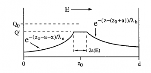
A diagram of the model is shown in Fig. 3 below. The charges surviving the cloud drift from the event center to the cloud radius, then experience the simple trapping effects as discussed above. The charges trapped in the cloud do not contribute to the measured signal since both carriers are assumed to diffuse uniformly.
| Figure 3 |
|---|
 |
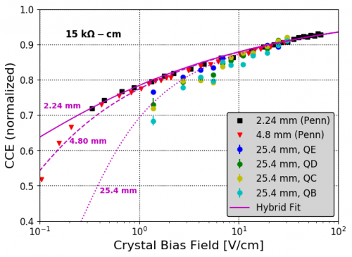
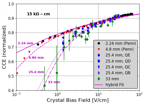
The model can be fit to the different datasets simultaneously using bias voltage and detector thickness as independent parameters. There are 5 parameters that must be fit. The results of such a fit are shown in Fig. 4 below and the parameters are in the table thereafter. All datasets have been renormalized by ~5% to match the high-field limit of the model. This adjustment is withing the 10-20% systematic uncertainties already present in both data sets. Fits are shown both with and without the UMN R60 data set which was somewhat noisy.
| Figure 4 | |
|---|---|
 |  |
| Hybrid Model Parameters | ||||
|---|---|---|---|---|
| Parameter | Description | Best Fit (No R60 data) | Best Fit (+ R60 data) | |
| b/L | Ratio of max cloud radius at F=0, b, to diffusion length scale <m>(L={\lambda_{step} \lambda_{trap}} / 3)</m> | 0.862 ± 0.018 | 0.851 ± 0.017 | |
| b | Max cloud radius at E=0 <m>(a=bE | {-n})</m> | 0.058 ± 0.045 cm | 0.065 ± 0.016 cm |
| n | Max cloud radius inverse Field exponent <m>(a=bE | {-n})</m> | 0.160 ± 0.007 | 0.146 ± 0.008 |
| c | Average capture length at E=0 <m>(\lambda=cE | m)</m> | 4.40 ± 0.911 cm | 2.76 ± 0.171 cm |
| m | Capture length field exponent <m>(\lambda=cE | m)</m> | 1.23 ± 0.283 | 1.13 ± 0.081 |
The model is a reasonable fit to the observed data. It gives a ~4.4 cm capture length with a ~linear field dependence. This is because the data shows no difference in trapping until the crystal is ~2.5 cm. The field dependence may be reasonable too. Penn et al. argue that <m>\lambda</m>~T~E in cold crystals. Cabrera et al. (2010) measured the carrier drift in Si and Ge and parameterized the average velocity with v~<m>E^{0.4}</m>, which gives <m>\lambda</m>~T~KE~<m>E^0.8</m>. So m~1.2 is not too crazy! The cloud radius is also consistent with Penn et al.'s measurements of b~0.01 cm and b~0.07 cm in samples of resistivities 2 kΩ-cm and 40 kΩ-cm respectively, though they obtained values of n~0.21-0.3.