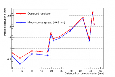
Table of Contents
Run 73 Summary
Detector channel geometry and source positions
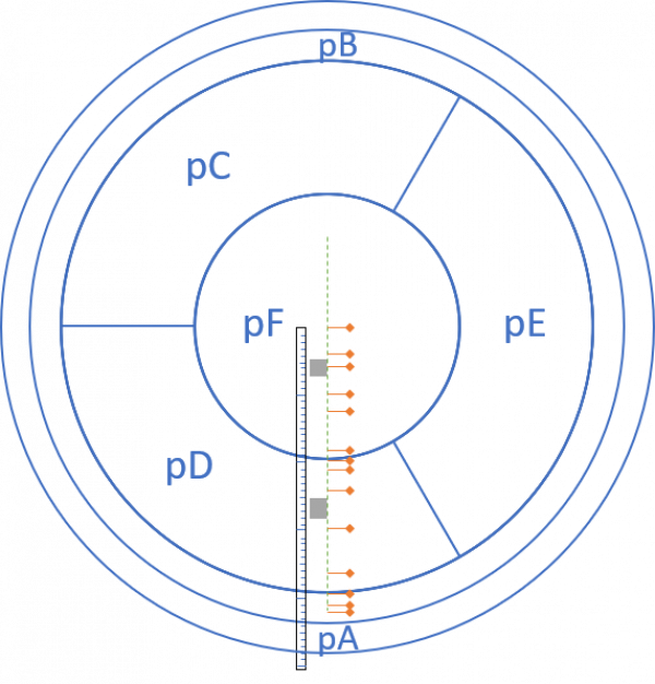
Confluence has info on the HV detector mask here: https://confluence.slac.stanford.edu/display/CDMS/100mm+HV+SNOLAB. It doesn't give the dimensions of the channels, but you can view the mask by downloading the .GDS file and using something called kLayout (a free download). This allows you to zoom in and see where the edges of the individual phonon channels are. In this way I found the following values:
| Channel | Inner radius [mm] | Outer radius [mm] |
|---|---|---|
| pA | 43.88 | 47.96 |
| pB | 39.32 | 43.75 |
| pC,D,E ring | 19.64 | 39.15 |
| pF | 0 | 19.55 |
Analysis planning
IbIs data
Data quality
Reduced gain
Early in the run we were confused that at 0V the gain was much lower than in Run72, and the pulse shapes bad (leading to far worse signal/noise). It turned out that the pi-filters had been left off of the readout cables - replacing them restored the gain and noise to levels similar to Run72. Comparisons linked below:
Polarity Differences at +/-10V
Data was taken starting at 0V for 4 minutes, then ramping to +10V and waiting 12 minutes, then lowering back to 0V and waiting 12 minutes. This was repeated with -10V.
| 0V (black), then +10V (red), then 0V (black) | 0V (black), then -10V (red), then 0V (black) |
|---|---|
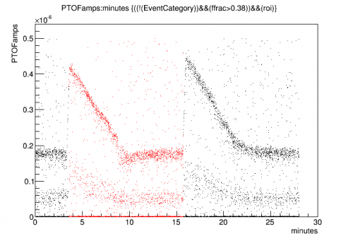 | 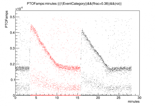 |
We can see the Luke gain fall to 0 as the counter-bias builds up. Then when the external bias is removed we can see the Luke gain return to nearly the same value as the detector self-biases, then it falls to 0 again.
Looking more closely it appears that at negative bias, the initial Luke gain is higher. For positive bias the initial Luke gain is lower, and as it falls to zero it undershoots the 0V gain level. This suggests some residual negative bias on the detector when the applied bias is 0V.
The minimum level of Luke gain is taken to be true-0V, which occurs at a point when the the positive bias is just high enough to cancel the residual negative bias. Using that assumption we can convert these plots to represent the effective bias on the detector, using the formula G_luke = 1+V/3.
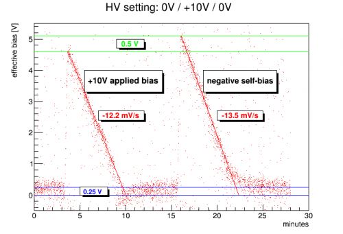 | 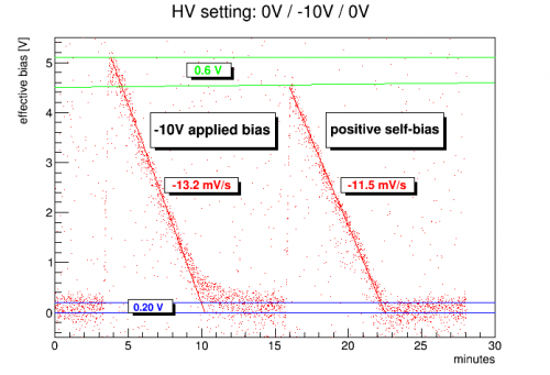 |
Judging from the undershoot, it looks like the residual bias is around -0.25 V, but judging from the difference between the highest points it looks more like 0.5 V.
Also noteworthy is that the falloff in Luke gain is faster at negative bias, suggesting that charge builds up faster on the surface at negative bias. Does this suggest extra charge leakage is occurring at negative bias? This would agree with the observed higher electron-equivalent noise at negative bias.
Charge leakage implications
Here's a closer look at the idea that the difference between Luke gain falloff rates for - versus + polarity is due to additional charge leakage at negative bias. On average, the falloff in effective Luke bias is 1.5 mV/s faster for negative bias. Suppose this were due to charge leakage? We can estimate how much charge is required to build up on the surface of the detector to produce a 1.5 mV bias in 1 second using the detector dimensions and the Ge dielectric constant (16). We find the following:
- Charge leakage current implied by 1.5 mV/s : 52 fA
This can be compared to an attempt I made to calculate charge leakage current in a completely different way - from the noise sigma seen when HV is applied versus noise at 0V. Below is a plot I showed at the Summer 2020 CDMS Collab Meeting:
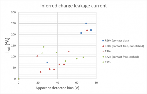
It should be noted that when this plot was generated there was considerable confusion as to the true detector bias during the contact-free runs (something I still want to sort out). However there is evidence from the negative bias points (the two open points) that leakage is worse at negative bias, and the charge leakage current implied at low biases is on the same order as the 52 fA calculated above. So it seems likely that the difference in Luke gain falloff between - and + polarity is indeed caused by differences in charge leakage.
Polarity Differences at +/-250V
On Sep 4 we took data at constant 250V, long enough for the NTL gain to fall to 1, then continued taking data after ramping the applied HV to 0. We did this in both polarities.
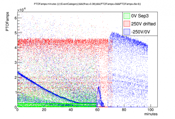 | 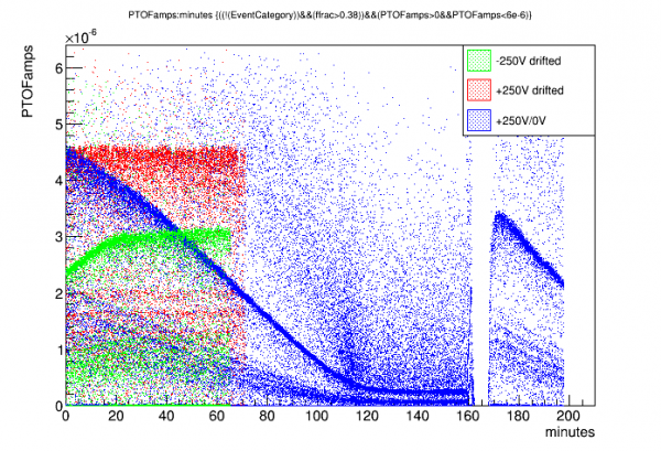 |
In each case we see the NTL gain fall from its initial value to a value consistent with 0V (NTL gain 1). Then during the rampdown there is an uptick and falloff in gain, followed by a period of no triggers, then when the applied HV falls to zero the gain quickly rises to a height equivalent to when the electrode is biased in the opposite polarity. (Note that the self-biased gain starts somewhat higher than the electrode-biased gain, basically consistent with a delay of around 10 minutes in the electrode-biased case, which is about right considering the prebias and rampup times.)
We can look at the rate at which the gain falls with time. Specifically let's calculate the NTL bias (that is, the apparent bias implied by the observed gain compared to the final gain) and plot the rate of change of NTL gain versus NTL gain. I use the 18keV line to do this - the 60keV line is of course easier but saturation strongly distorts the gain at high bias (there may still be some saturation at high bias at 18keV).
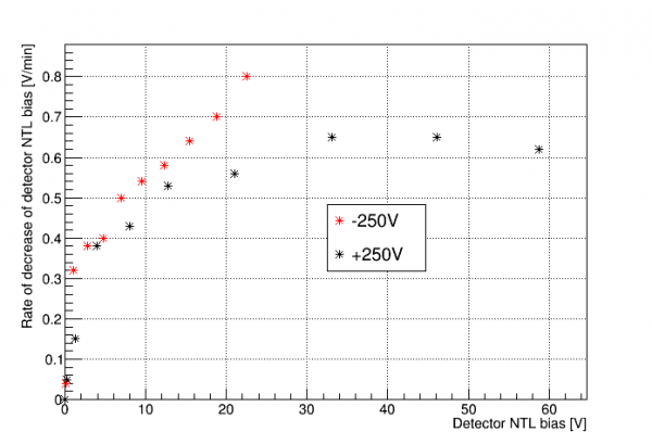 |
This gives an indication of the rate at which surface charge builds up in the detector, producing a counterbias. Exactly how to calculate this bias depends on the model you choose for why the NTL gain is what it is - and it's not yet understood why it is so much lower than expected and why it is so different in negative versus positive polarity. Regardless, we can assume that this current is a combination of charges produced by events and charge leakage. Note that both polarities seem to point to the same point on the y-axis (ignoring the near-zero points), suggesting that this is the rate of change based on events. The additional rate seen at higher biases then comes from charge leakage, with the leakage being worse for -bias.
Run plan for August 22-30 (Matt on vacation)
- Continue taking drifted HV data at higher biases, both polarities
- We have gone as high as +75V, -75V (tried +100V but it was a bad data series). See dataserieslist.xlsx
- So far we have not seen the much-lower Luke gain in -bias that we saw in previous runs. Definitely saw it at -300V in previous runs. We should keep going and look for this phenomenon: +/-100V, +/-150V, etc.
- Use the Excel spreadsheet to make new sequences for drifted data (sheet “drift_w_prebias” in “Run73IbIs.xlsx” on fridge computer in K100electrical folder)
- option: either use prebias or don't. We've seen evidence that prebias reduces noise a bit, so probably use it. Standard: 75% for 2 minutes.
- The drift rate necessary for constant gain seems to increase as we increase the bias. There's an Excel spreadsheet (run73_Lukegain.xlsx) to keep track, and to guess what drift rate is necessary for the next bias.
- Look at data - if gain is not constant, try again with adjusted drift rate. Example analysis script
- For our good data so far, triggering on DCRC1pD (Side1pF) with threshold=8 works fine. We've had some bad states though, with spiky noise - in those cases you need a higher threshold. Or you need to try to “fix” the problem somehow (check Ebox purge; reboot DCRCs; etc?)
- Basic steps to powercycle DCRC: turn off DAQ programs triggerfe2, towerfe3_01, dcrc_driver01. Unplug ethernet power from DCRC. Wait maybe 30 seconds, then plug back in. Restart DAQ programs in reverse order. Zap SQUIDS on the DCRC(s) that were restarted.
- Monitor “lag ratio”. Recently it has been very consistent. Use the HV plot from OmniLogger to determine when the drift begins and ends. This time span divided by the nominal drift time (our default is 60 minutes) is the “lag ratio”. It has been consistently 1.10. If it's different from this, then it will be harder to get the drift rate right.
- Monitor the HV current leakage. Check Vtest at beginning and end of drift. Quick formula: HVlossfraction=0.4*Vtest[mV]/HV[V]. This loss fraction should be around 2% or less if the Ebox purge is working.
- The meter that monitors the HV has a maximum, I'm not sure what it is (400V maybe). If we keep increasing our HV drift settings we will eventually hit this maximum. When that happens we should probably stop using that meter, unplug the banana cables connecting HV to the meter.
- QET biases: if we take data at the same temperature every time, we can use standard settings. If the temperature isn't consistent, we should adjust. I made a table for QET bias settings at different temperatures that should keep the TES gains (dI/dP) roughly constant between data series at different temperatures. (Not sure how temperatures will be now that I've changed the mixture.)
- so far in the run, temperature increases to mid-to-high 50s after LN2 fills, slowly cools to low 50s.
- Source mover data
- Not sure we'll have time to get to this this week
- We should choose a specific HV to use for position-dependent data (highish positive bias)
- Should probably try a series of 4-step moves with 4-min pauses, like Run 71
- After moving to a new position, we can again check to see if there's a reduction in gain (through loss of phonon collection efficiency (PCE))
- To restore PCE we need to do “hot Al flash” (then take more data to make sure it worked)
- Data Processing and Monitoring
- After a data series is complete, it should be added to the Data Series List (online spreadsheet)
- Zach will process the data series after they are finished.
- Path to Zach's processed data: /data/chocula/will/data/k100proc/midasrq
- Need someone to do quick analysis, at least PTOF-versus-time to see whether the 60keV line is flat
- If there are problems contact Matt:
- should be available by email and Slack usually
- also feel free to call, 612-232-0422
- Vuk's number: (510) 703-4343
Channel balancing and Am-241 selection
Source Mover Position Analysis
Channel Delay
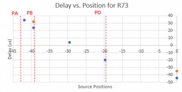
The delay data come from several series at various positions from the center to near the outer end stop (-42 mm) all at 300V bias. The delays are calculated from the following alias:
pdelWK = -1e6*(PAWKr30 - PFWKr30)
This makes use of the 30% risetimes of the events in the series, here it's normalized to units of us and set so a negative value corresponds to events with lower delay in F and a positive value corresponds to events with a lower delay in A. Below is a rough estimation of the delay values with the channel boundaries plotted in vertical dotted lines, there are two positions, 0 and - 39.4 mm that have two data points since the main peak in the delay spectrum was split.
FAIR project machine-learning results
r73-fair-initial_results.pdf
More position reconstruction
This section will approach position reconstruction with the intent of comparing to the machine learning results.
Data provided to the FAIR project for machine learning:
- 13 different source positions, data at +300V
- Am-241 events selected by partition, 14keV and 18keV peak events selected
- Attempt at channel balancing within series and amplitude balancing across series
- RQs provided, for all 5 channels: adjusted OF amplitude, 20% risetime, 40% falltime
- “Truth” information provided: source position, energy (13.95 or 17.74 keV)
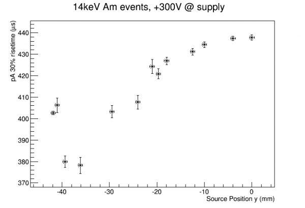
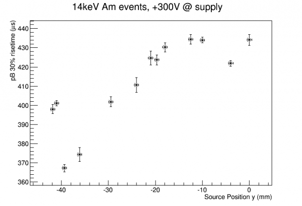
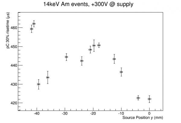
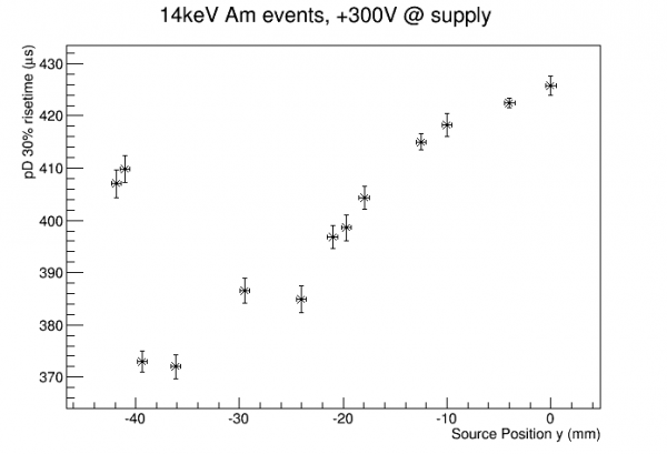
As a first look here are raw risetimes for the 14keV events:
 |  |
 |  |
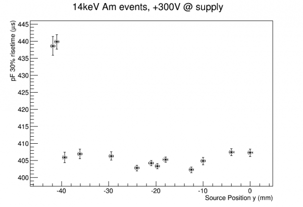 |
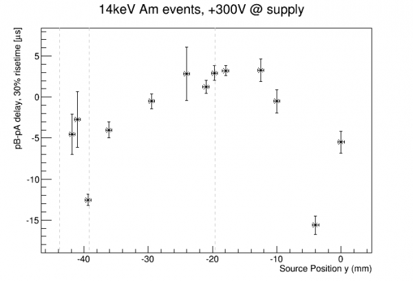
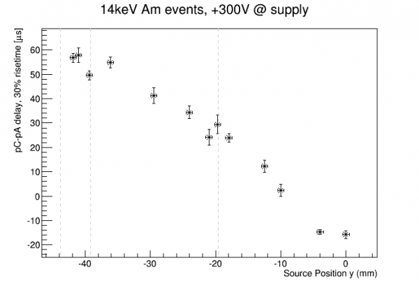
An odd feature of these plots is that for every channel the two leftmost points (which are from the last two series taken) seem to jump to later risetimes than the overall pattern suggests, all by about 35 μs. Is this actual detector physics? No - checking the run diary shows that the trigger scheme was changed for these last two series. The first 11 series were all generated by triggering on pF only, but for the last two we decided to trigger on pF or pA. As can be seen from the plots, at the higher radii pA rises sooner than pF, so when we include pA for triggering it will catch the event sooner, and thus all the pulses will appear later in the trace.
This information should not be provided for the machine learning projects, because it biases the two positions closest to the edge by changing the DAQ (of course position reco should depend on the detector response, not the DAQ configuration). The only physically relevant quantities are the relative delays. So instead of providing risetimes for each channel, we should provide delays with respect to some standard for the event. The only unbiased standard available is one of the risetimes themselves (or arguably an OF time?). So we can use pA as a standard (as we do in channel balancing) and provide risetime delays for the other 4 channels wrt pA. Similarly we don't want to provide raw falltimes either, they will be biased in the same way. So rather than falltimes we can provide widths, falltime-risetime for each channel (pulse width was the main motivation for providing falltimes to begin with). Originally I packaged these raw quantities, figuring that the machine could construct whatever delay-like or width-like combinations it wanted, but clearly there's a problem with that.
Below is a look at delays wrt pA for the 14keV events:
 |  |
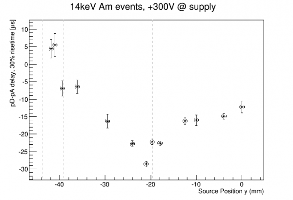 | 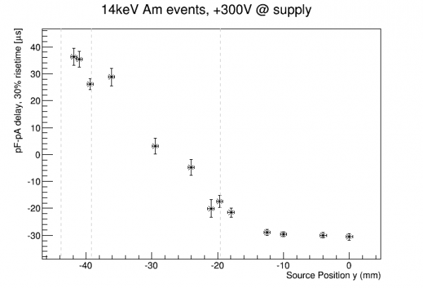 |
We can go ahead and try to do a simple position reconstruction based on one of these quantities. The pC delay looks like it has the most sensitive and monotonic response to position across the full range. Below I invert the plot and fit to a functional form; sinh seems to give a simple enough fit.
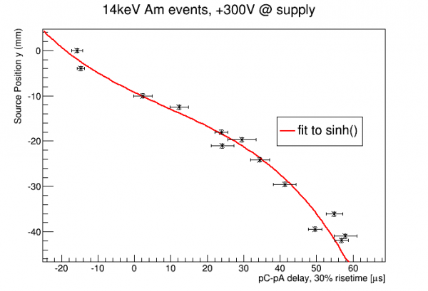
We now have a position reconstruction based on the pC delay. We can see that some points are more on the curve than others. Since this delay quantity should be fairly robust these are probably real effects of detector physics, and in principle we could have a fit function with more parameters. But we don't have enough points to really see those variations well so we'll stick to this simple 4-parameter function.
The error bars in pC delay in the above plots are based on Gaussian fits. Below are some attempts to give a more complete view of the position reconstruction performance by looking at complete distributions:
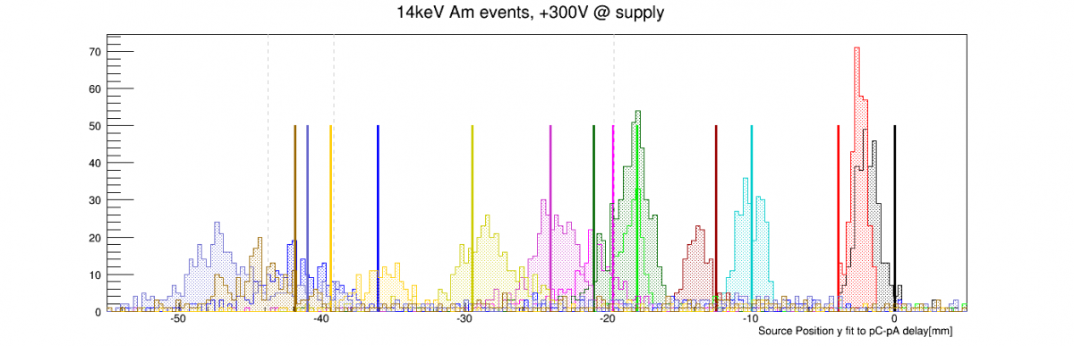
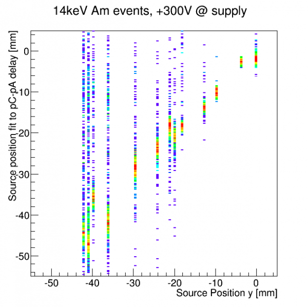 | 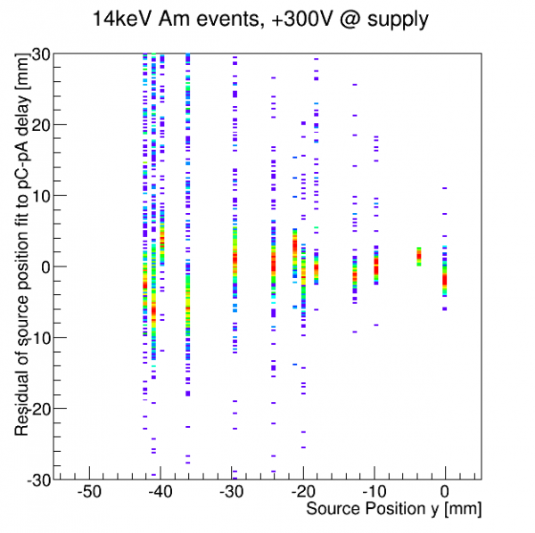 |
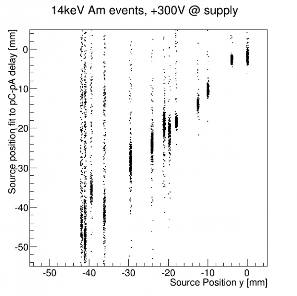 | 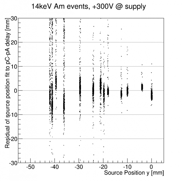 |
These don't look too bad. Now let's try to compare to some of the machine learning results. Taihui used the mean-square-error, MSE, as a figure of merit for the ML models. For each source position, he took the predicted positions for the events from the position dataset that was not trained on, and took the mean of the squared differences between the predicted positions and the truth value. This means that the MSE combines two errors: the statistical spread of the distribution around its mean (RMS), and the systematic shift between the mean of the distribution (offset). The MSE is the sum of the squares of those: MSE = RMS^2 + offset^2. In some cases Taihui's MSEs are dominated by RMS, in other cases by the offset.
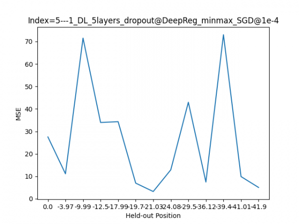 | 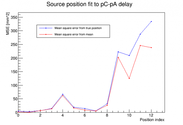 |
On the left are the MSEs for one of Taihui's better-performing models. On the right are MSEs similarly calculated from my pC-delay-based reconstruction. Also in the plot on the right, in red, are squared errors around the mean. So the red itself represents the statistical spread, and the difference between the blue and the read represents the systematic offset.
Since Positions 9-12 have such large MSEs this would probably be categorized as a failure among the machine learning models. But does this reconstruction really perform that badly? It doesn't look so bad when you look at the distributions. (At least not to a particle physicist…)
The plot below shows the distribution of deviation between reconstructed and true position for Position 9, which has a rather bad MSE value:
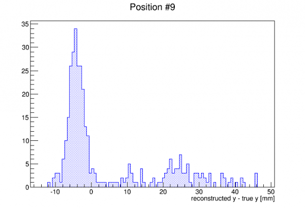
The MSE is driven by the outliers. There are pretty many outliers, but there is also a prominent peak. Of course particle physicists are trained to focus on the peak - they are used to peaks sitting on top of background. A more natural figure of merit to a particle physicist would be based on a Gaussian fit to the peak. (As mentioned the error bars I generated for the pC delays were based on Gaussian fits.) Below is a plot similar to the MSE plots above, but based only on the Gaussian fit to the peak:
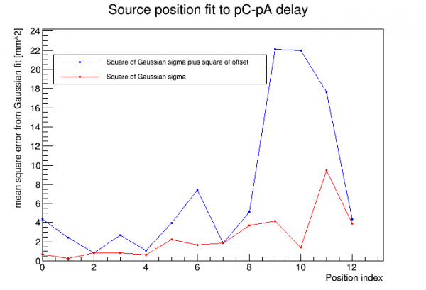
This looks much better, and for the purposes of the physical problem at hand this is a better description of the reconstruction's performance. This indicates the ML models won't recognize a good result when they see it.
What about these outliers? Examining the events reveals no pathologies - they are not pileup or tail events, they look good. These are likely good background events that have slipped through the rough selection cuts for Am-241 events. (The distribution of outliers supports this - they seem to be spread across the natural y-range.) Since these cuts are more difficult to do at high radius positions, we wind up with more outliers in the last few positions, and thus bad MSE values for those.
How do we improve the machine learning result? The most obvious answer: do more thorough Am-selection cuts to remove background. We can for example do a 2-sigma or 3-sigma cut on pC delay itself. If we want to avoid bias we could do this on every quantity.
The other way to improve the machine learning model would be to set it up to optimize not the MSE but rather to focus on the “peak” and to de-emphasize outliers. I don't know how doable that is.