Table of Contents
Channel Balancing and Am-241 Event Selection
First look at balancing and partition-based selection
In this section I look at 300V data at five different source positions:
| 0 mm | Center of pF | 07200831_2206 |
| -19.7 mm | pF / pD interface | 07201013_1643 |
| -29.5 mm | Middle pD | 07201017_1636 |
| -39.4 mm | pD / pB interface | 07201023_0633 |
| -41.9 mm | Middle pB | 07201027_2114 |
To explore the partition space I chose to plot two-channel fractional partitions. In all cases I use pA as a reference channel: the x-axis is PAOFamps. On the y-axis I plot B*pX/(pA+B*pX), where pX is one of the other channels and B is a balancing factor. I adjusted the balancing factors so that events not in the Am peaks are roughly centered around 0.5 - i.e. the assumption is that for uniformly distributed events there is on average equal energy in pX and pA. This may not be physical but as a standard it should at least put each different series on an equal footing. (In other words the imbalance between channels should be the same in every series.) Also for each series the x-axis scale has been adjusted to fit the maximum pA amplitudes.
The row labeled “bal” shows the pB / pC / pD / pF balancing factors used. The row labeled “pA range” shows the maximum value of PAOFamps used in 1e-6 units - roughly speaking this is an inverse overall balancing factor for all channels.
| 0 mm | -19.7 mm | -29.5 mm | -39.4 mm | -41.9 mm | |
|---|---|---|---|---|---|
| pB | 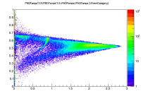 | 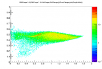 | 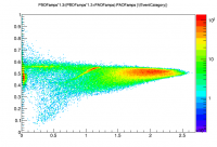 | 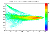 | 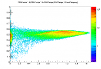 |
| pC | 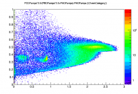 | 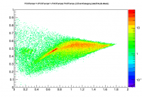 | 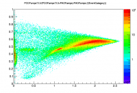 | 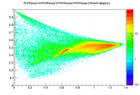 | 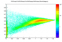 |
| pD | 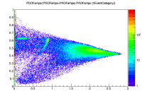 | 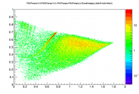 | 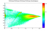 | 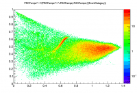 | 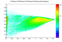 |
| pF | 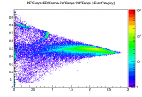 | 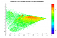 | 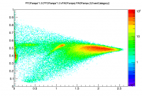 | 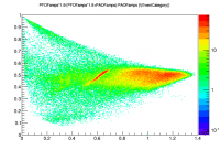 | 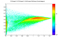 |
| bal | 2.2 / 2.5 / 1.0 / 1.0 | 2.5 / 7.0 / 2.2 / 2.0 | 1.3 / 2.3 / 2.0 / 1.2 | 1.2 / 3.0 / 1.7 / 1.9 | 1.4 / 3.5 / 2.0 / 2.7 |
| pA range | 3.0 | 2.0 | 2.7 | 1.4 | 1.7 |
First let's look at how the apparent balancing factors vary over these five runs. Or rather the inverse balancing factors, taken to be relative gains. Here I use the different pA ranges to infer the pA gains then scale the relative gains of the other channels to that for each series.
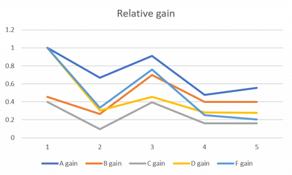
Gains seem to vary a lot, both between channels and over time. The last two series are relatively similar. These two series were taken after I had started inferring the detector temperature as a function of tower thermometer determined by doing repeated IbIs measurements, and adjusting QET bias constantly based on the inferred temperature. For the third series I was already adjusting QET biases constantly, but using the unadjusted tower thermometer readout. The next day was when I decided the tower thermometer was not accurately giving the detector temperature.
By the time the last two series were taken (at least) I was setting QET biases so that the gains according to IbIs of all channels were equal. Clearly the empirical gains are not equal. But these calculations are based on the assumption that on average uniformly-distributed events will deposit equal energies in all channels. It's possible the A-ring and B-ring channels actually absorb a larger share - if so that would explain why their gains appear higher than the other channels. But certainly pC and pD should have the same gains - they clearly do not. pC has the lowest gain in every series, which was pretty noticeable from the pulse viewer during the run. It makes me wonder whether that channel is actually damaged somehow.
Identifying Am-241 events
The plots above are adequate for locating the Am-241 events. The 60keV line is obvious in all series but it seems to be pretty distorted - at 300V it is surely quite saturated which is probably part of the reason for that. So we focus on the lower lines, particularly 14 keV and 18 keV.
The pF fraction plot is obviously the best for selecting Am-241 in the first series (y = 0 mm, center of pF). But for all other series in this note, starting at the inner edge of pD and working out to pB, it seems that the pD plot is best.
The cuts below are decent at selecting the lower Am-241 lines, and also catch a little of the 60keV line:
	TCut cam[5]
	cam[0] = "PFOFamps/(PFOFamps+PAOFamps)>0.7"
	cam[1] = "PDOFamps*2.2/(PDOFamps*2.2+PAOFamps)>0.68"
	cam[2] = "PDOFamps/(PDOFamps+PAOFamps)>0.62"
	cam[3] = "PDOFamps*1.7/(PDOFamps*1.7+PAOFamps)>0.60&&PDOFamps*1.7/(PDOFamps*1.7+PAOFamps)<0.72"
	cam[4] = "PDOFamps*2/(PDOFamps*2+PAOFamps)>0.55"
The 4th series in this list (cut cam[3]) is the most complicated, in that the Am events seem to fall in a middle range of pD fraction rather than at the top. That's the series with the source on the pD/pB border.
Using these cuts, decent Am spectra can be drawn in PAOFamps. (Throughout this note I'm avoiding PTOFamps since the balancing is so out of whack.) The spectrum is quite sharp for the first series, but just OK for the 2nd, 3rd, and 4th. For the 5th series I used a correction to PAOFamps based on the slope of the 18keV line seen in the pD fraction plot, in order to make those lines vertical in the plot. (This is based on the observation that events in the peaks with a low pD/pA ratio also have a relatively low pA amplitude; in other words the amplitude of some of the events in the peak seems to be low overall, but the damping is greater in pD than pA, which gives a handle for correcting them. Why this is I have no idea.)
The plots below are the same channel fraction versus pA plots as above, with selection cuts for the 14 keV and 18 keV highlighted in magenta and red, to give a better idea of where these events appear in each channel.
| 0 mm | -19.7 mm | -29.5 mm | -39.4 mm | -41.9 mm | |
|---|---|---|---|---|---|
| pB | 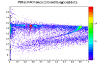 | 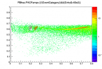 | 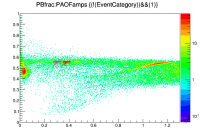 | 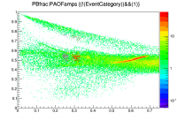 | 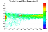 |
| pC | 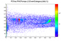 | 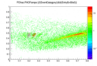 | 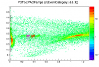 | 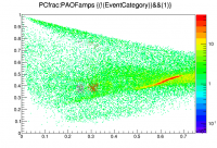 | 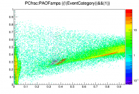 |
| pD | 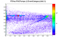 | 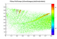 | 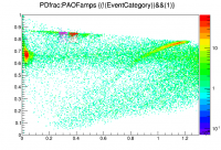 | 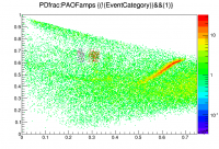 | 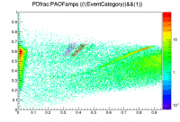 |
| pF | 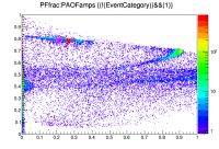 | 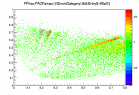 | 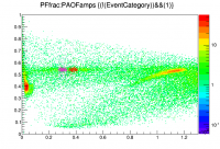 | 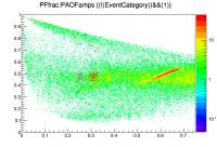 | 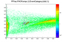 |