Table of Contents
NaI Detectors
First Look
This run features 2 NaI detectors mounted on the south shield wall. They will act as coincidence detectors and will be used to search for high energy gammas from nuclear de-excitations in the CDMS detector. The NaI detector bias of 1.1kV and signal amplification are provided by NIM modules. The NaI pulses are digitized by a DCRC's phonon channels. The first background spectrum taken with this complete setup is shown below. The upper detector is detector B and the lower is detector C.
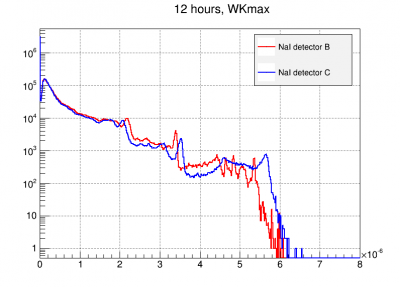 |
| Preliminary NaI spectra digitized by DCRC4 Note: Detector labels are wrong in this figure. B↔C |
The plots below show the energy quantities change discretely over time, resetting at the beginning of each run. The structure in detector B seems to be present after such 'resets'. The only way we know to mitigate this is by taking shorter sub series.
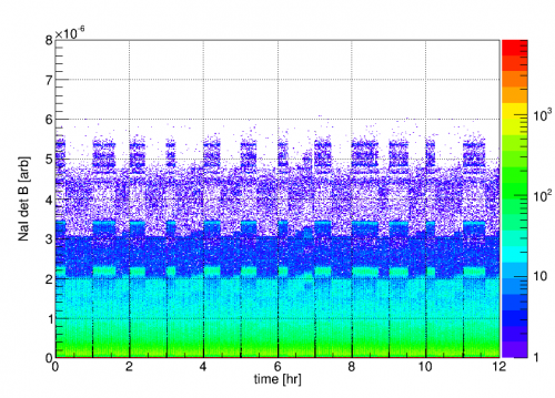 | 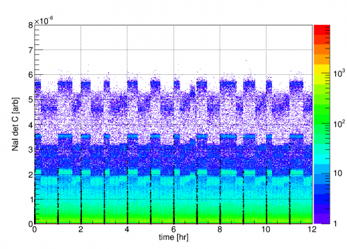 |
| NaI detector signals vs. time. Randoms at the beginning of each series are highlighted in black. Note: Detector labels are wrong in this figure. B↔C |
|
It turns out the structure seen in detector B is associated with large pulses which ADC rail. Since the WK algorithm does some basic filtering, presumably the different bands observed have something to do with width of the flat pulse top interacting with the filter. This should be avoided by reducing the amplifier gain and adjusting the driver offset.
These events should be cut by using the P*sat RQ. However it does not seem to be working right. C.F. Series 07180814_1139, events 90546 (Large pulse ADCmax=16383, PAsat=0) and 91838 (glitch bin ADCmax=20803, PAsat=1).
Update 8/22
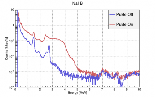
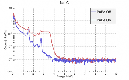
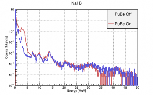
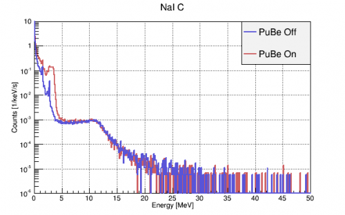
PuBe On/Off spectra calibrated to (0, 0.511, 1.275, 1.461, 2.615) MeV lines from a dedicated calibration run. PuBe should have a ~4.44 MeV gamma that may be causing the large shoulder. Structure is still observed above 5 MeV in detB but is apparently not ADC saturation. Perhaps it could be real signal that is smeared by detC's amplifier? 207Pb (22% abundance) does have a prominent 7.4 MeV capture gamma, but that shouldn't be present in the PuBe Off data. We are not yet sure what all the other structure could be.
 |  |
 |  |
| Note: Detector labels are wrong in this figure. B↔C | |
Update 9/25
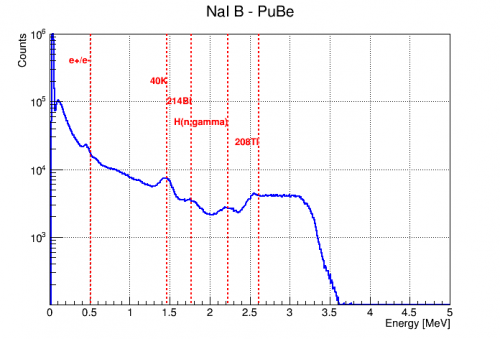
It was realized late in the run that the NaI amplifier input polarities were set to “pos” when they should have been “neg” since the incoming NaI signal was negative-going pulses. Using the correct polarity improved the NaI signal linearity, but did not appreciably change the spectrum above ~3MeV. The resulting spectrum of detector B was calibrated linearly and is shown below.
 | 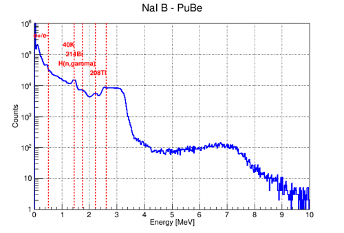 |
Detector C also became more linear with the polarity correction, but the spectral structure above ~4MeV remained. A spectrum was also taken using another amplifier with similar results below 2 MeV, but a stronger 2.6 MeV peak and different structure above 4MeV as seen below.
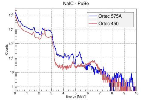 |
It was also found that the NaI spectra were slightly different for the two detectors, even when measured through the same amplifier and digitizer.
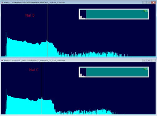 |
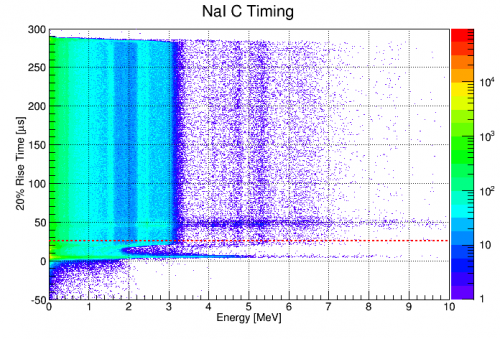
There was some confusion early on about the shape of the NaI pulse timing distribution. A deviation in this distribution was particularly clear in the pulse start time vs energy plane (seen below). However, it was found to simply be an effect of the DC baseline subtraction done on all pulses as the first step of processing. For the NaI detectors, the first 32 bins (25.6 us) are used to calculate the trace baseline, which is then subtracted. Thus, pulses that have some portion in this window will be shifted incorrectly and have garbage timing and amplitude calculations. This necessitates a cut on all NaI traces having a start time before 25.6us.
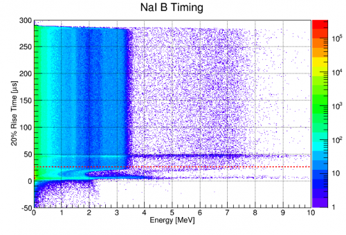 |  |
Corrected Bias, Dynode Termination, and Amplifier Study
As described on 2018/09/26, two issues were discovered in the NaI setup. The first was that the PMT bias had been set to 1.2kV instead of 1.1kV for the majority of the run. Reducing this brought signals above ~3MeV into appropriate amplitude ranges for the amplifiers. The second was that the PMT dynode should be terminated when not in use. Putting 50Ω terminators on them seemed to further improve the high energy range of the NaI spectra.
An example of the result of dynode termination is shown in the spectra below. Both were taken at 1.1 kV PMT bias, the Ortec 452 amplifier, and with the PuBe source to the south of the fridge. The only difference is the termination of the unused PMT dynode terminal with a 50Ω terminator. It is clear that leaving the dynode open greatly distorted the high energy signal.
 |  |
Some spectra were taken with these new settings (1.1 kV, terminated dynodes) and 3 different amplifiers to identify the optimal arrangement. The amplifiers tested were:
- Ortec 450 (Neg Input, G=5*1, shaping=5us integrate, Output Range=+10V)
- Ortec 452 (Neg input, G=5*2.5, shaping=6us, Output Range=+10V)
- Ortec 575A (Neg Input, G=2*2.5, shaping=3us)
All amplifiers were followed by x10 attenuation and digitized with the Ortec EasyMCA and Maestro with livetimes around 400s.
This set of plots shows the NaI detector B spectrum through the three different amplifiers. Each plot shows the spectrum with the PuBe source near the south lab wall and with the addition of the 22Na source to corroborate line identification.
| NaI B, Ortec 450 | ||
|---|---|---|
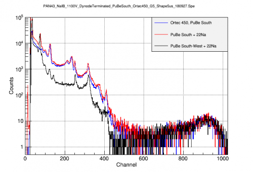 | 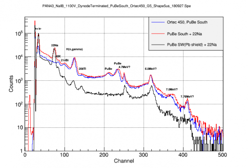 | 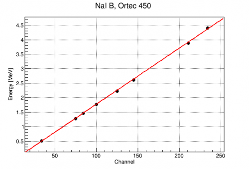 |
| By comparing source arrangements, the 22Na lines can be identified at 0.511 and 1.275MeV, as can the 4.4MeV PuBe line and it's single escape peak. A second line is resolved at 4.7MeV as are several others as high as 7.8MeV. Again the calibration is quite linear for known lines. |
||
| NaI B, Ortec 452 | ||
|---|---|---|
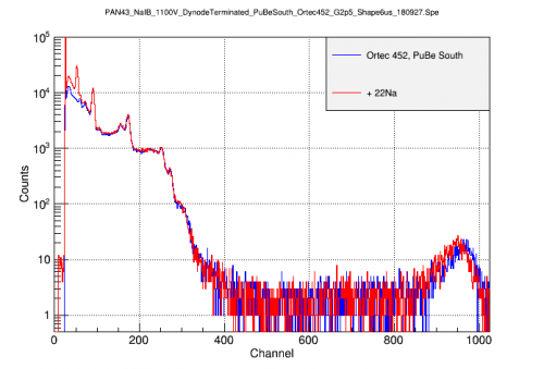 | 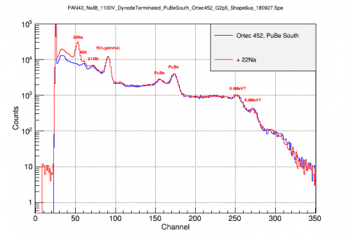 | 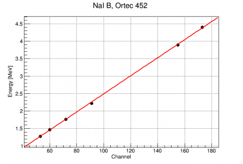 |
| The 1.275 MeV line of 22Na is clearly seen at Channel 53. From this, the 2.2 MeV Hydrogen capture and 4.4 MeV PuBe lines can be identified. There seem to be additional lines visible out to at least 7MeV The calibration is quite linear out to at least 4.4MeV |
||
| NaI B, Ortec 575A | ||
|---|---|---|
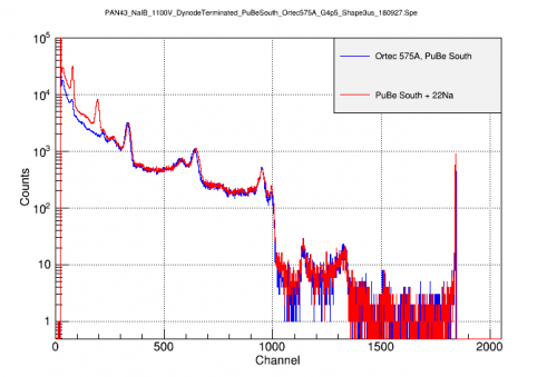 | 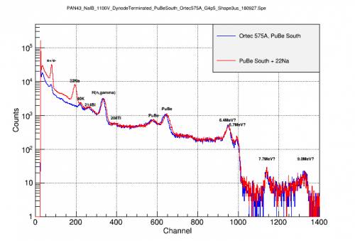 | 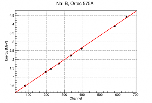 |
| Note the signal amplitudes are more than twice the Ortec 450 with same gain, perhaps due to the shorter shaping time. The amplifier appears to have a hard saturation near channel 1850. By comparing source arrangements, the 22Na lines can be identified at 0.511 and 1.275MeV. All lines up to the PuBe 4.4 MeV are identified. Higher lines appear, possibly up to 9MeV. Again the calibration is quite linear for known lines. |
||
After identifying the lines below 4.4MeV, the spectra from the three amplifiers can be calibrated and compared. The most troubling feature is the two peaks at 4.7 and 6.0 MeV only seen with the Ortec 450. These have not been identified as physical peaks. They also appear in spectra digitized with the DCRCs, but the individual traces do not appear significantly different from other events (okay baseline, normal height/integral ratio). However, their resolutions are suspiciously narrow and the structure at 6MeV has a shape suspiciously like a resonance peak. These facts make one suspicious that these are noise/glitch artifacts from this particular amplifier (Ortec 450). Accordingly, the amplifier should be replaced and any data taken with it treated carefully.
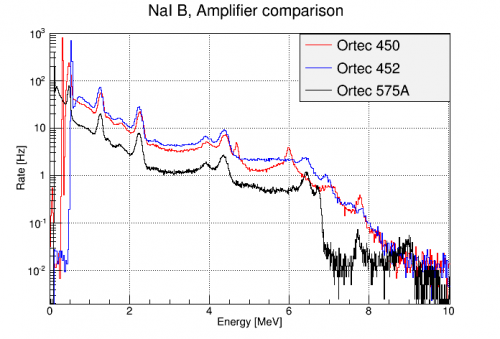 |
| The three amplifiers agree up to 4.4 MeV. Above that, however, the Ortec 450 has suspicious peaks not seen with other amplifiers. |
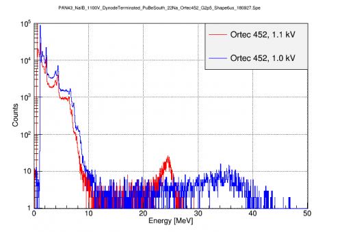
Even with the PMT bias lowered to 1.1kV, some of the higher lines (>6MeV) may still be saturating the amplifier. This can be seen by comparing to a spectrum taken at a still lower PMT bias of 1.0 kV. At this bias (1.0 kV), the 511 keV line starts to fall below threshold, but the signals from higher lines should fall closer to the amplifier's linear range. This can be seen in the figure below. In the 1.1 kV spectrum, the calibration up to 4.4 MeV was seen above to be linear. This indicates the amplifier's response is linear up to Channel 175. Assuming the NaI and PMT response are linear, this would mean we can use a linear calibration in the 1.0 kV spectrum to identify the three higher peaks.
 |
Below are the two spectra after a linear calibration is applied to each. Both agree up to 4.4 MeV, but above that the 1.1 kV signals start to be reduced compared to the 1.0 kV. Based on the 1.0 kV calibration, the 3 high bumps have energies of 6.65, 7.28, and ~8 MeV. These have not yet been positively identified.
 |  |
PuBe gamma flux estimate
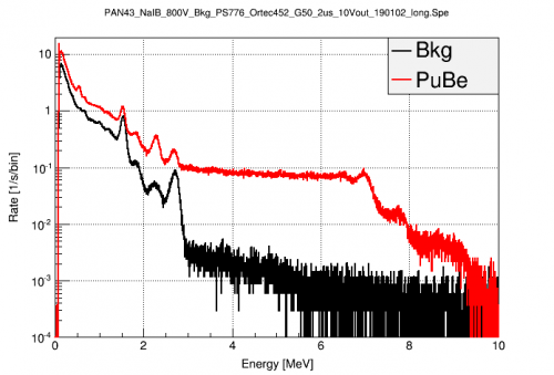
Triggered PuBe data was taken on 2019/01/02 in order to study the effects of PMT bias and to quantify the flux of high energy PuBe gammas which might contribute to a coherent gamma-nuclear scattering signal in the HV detector. Some of the calibrated spectra taken that day were used in the following plots. The spectra were taken with the NaI B detector mounted in it's standard position, biased at 800V, with the PS776 preamp, Ortec 452 amplifier (neg input, G=50, +10V out, 2us), and digitized with Easy MCA. They were calibrated to the known lines with a single scaling factor of 1/307.651 MeV/channel.
The first figure compares the background and PuBe spectra with the PuBe source in it's standard location behind the large Pb wall. The 4.4 MeV direct gammas are strongly suppressed relative to the other high energy gammas present with the source in place.
 |
The next figure shows the integrated rate of these events above a given energy. The x-axis is the lower limit of the integral. This is in units of events/s interacting with the NaI detector.
 |
We can use this to estimate the flux of such gammas at the HV detector. To do so, we'll scale the measured flux using the detector geometries. One extreme is to assume that all of these gammas are coming from the direction of the PuBe source, so the cross-sectional area of the detectors (diameter*height) is the appropriate measure. The other extreme is to assume the majority of these high energy gammas are actually from (n,gamma) processes in the shield or fridge material, so the total detector surface area is more appropriate. The relevant measurements are shown in the table below.
| Detector Geometries | ||||
|---|---|---|---|---|
| Detector | Radius [in] | Thickness [in] | Surface Area [in^2] | Cross-section Area [in^2] |
| NaI | 4 | 8 | 250 | 64 |
| HV | 2 | 1.3 | 29 | 5.2 |
Using these values, the ratio of surface areas of the NaI/HV detector is 8.6 while the ratio of cross-sections is 12.3. If we use these to scale the flux plots above to that expected for the HV detector, we get the figure below.
 |
Here we see that the estimated rate of high energy gammas towards the HV detector is 10s-100s of Hz. This seems rather high given that the observed event rate in the detector is ~1-10Hz, but at these energies, the penetration depth of the gammas is 10s of cm, so they may be unlikely to interact with the HV detector much.
PuBe Calibrations in Triggered R68 Data
The NaI detectors were calibrated for all of the R68 -125V datasets. The corrected WKmax amplitudes were used. The detectors were generally calibrated using the following identified gamma peaks (when present): e-/e+, 40K, 214Bi, n-capture on H, 208Tl. The details of the calibration are in the following file: /home/mast/cdms/analysis/run068/r68_n125_NaI.c . The resulting calibrations are below:
z_bkg->SetAlias("NaIBMeV","(dataset==1)*(0.0305279+NaIBWKmax_corr*1.20282e+07) + (dataset==2)*(0.0159196+NaIBWKmax_corr*1.71157e+07)");
z_bkg->SetAlias("NaICMeV","(dataset==1)*(0.0319984+NaICWKmax_corr*6.36238e+06) + (dataset==2)*(0.00553167+NaICWKmax_corr*5.78771e+06)");

z_Na->SetAlias("NaIBMeV","(dataset==1)*(0.0253436+NaIBWKmax_corr*1.05725e+07) + (dataset==2)*(0.00864543+NaIBWKmax_corr*1.69852e+07)");
z_Na->SetAlias("NaICMeV","(dataset==1)*(0.0113478+NaICWKmax_corr*6.82094e+06) + (dataset==2)*(-0.00255718+NaICWKmax_corr*5.77976e+06)");

z->SetAlias("NaIBMeV","(dataset==1)*(0.0371032+NaIBWKmax_corr*1.01686e+07) + (dataset==2)*(0.0424504+NaIBWKmax_corr*1.06675e+07) + (dataset==3)*(0.019922+NaIBWKmax_corr*1.1006e+07) + (dataset==4)*(0.0187856+NaIBWKmax_corr*1.68475e+07)");
z->SetAlias("NaICMeV","(dataset==1)*(0.0188233+NaICWKmax_corr*3.55224e+06) + (dataset==2)*(0.0265557+NaICWKmax_corr*6.84554e+06) + (dataset==3)*(0.0170364+NaICWKmax_corr*5.69084e+06) + (dataset==4)*(0.0193087+NaICWKmax_corr*5.6491e+06)");
The accuracy of these calibrations varies across different datasets, but they are generally trustworthy up to at least 2.6 MeV. With these calibrations, we can investigate the effect on the HV spectrum of requiring coincidence in one of the NaIs. The details of this analysis are in : /home/mast/cdms/analysis/run068/r68_n125_spectrum_wNaI.c
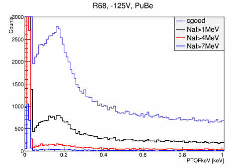
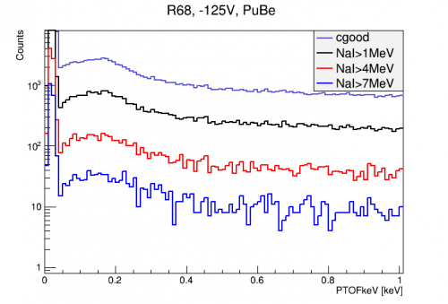
The figure below shows the effect of imposing NaI coincidence cuts on the HV detector spectrum with all final quality cuts applied. The NaI coincidence cuts require that one of the NaI detectors had an event above the given level within 100 us of the HV detector trigger time. There is a considerable fraction of events at all energies that are removed by this cut. Interestingly though, there may be hints of two peaks in the capture signal with the 1 MeV cut.
 |  |
It is important to understand what passage fraction we expect from this cut simply from accidental coincidence. Since randoms are uncorrelated with the NaI detectors, they give a good estimate of the rate of accidental coincidence with the HV-triggered events. The fraction of random events which are paired with an event in one of the NaI detectors above a certain energy are shown in the table below.
| NaI over: | Fraction of Randoms |
|---|---|
| 1 MeV | 0.276 |
| 4 MeV | 5.34e-2 |
| 7 MeV | 1.00e-2 |
| 9 MeV | 4.60e-4 |
We can then compare to the average passage fractions for several energy ranges of triggered data:
| Fraction of Triggered Events | |||
|---|---|---|---|
| NaI over: | 0-0.5 keV | 0.5-2 keV | 0-2 keV |
| 1 MeV | 2.90e-01 | 2.80e-01 | 2.82e-01 |
| 4 MeV | 5.18e-02 | 5.72e-02 | 5.27e-02 |
| 7 MeV | 1.19e-02 | 1.31e-02 | 1.21e-02 |
In general the passage fractions are a little higher than the accidental rate, indicating there is some correlation between the HV and NaI detectors. So if the fraction of (n,gamma) events that send a gamma to the NaI is low, we may not see a strong excess passage fraction for those energies. Around 7 MeV, where we expect some gammas from capture, there is an excess of ~0.2% which may be the (n,gammas). Our naive estimate for this fraction is ~1% just from solid angle. It could be 0.2% due to shielding and absorption probabilities. This can be verified with simulation and may be useful for obtaining a better sample of (n,gamma) events.