Table of Contents
Run 76 Analysis: Electron-equivalent Energy Calibration
Example (Matt)
Step 0: Load data and baseline correction
Before calibrating high-voltage, high-rate data you first need to correct energy for baseline as described in the baseline correction note. Below I use the same example data and repeat all the code needed for the baseline correction:
gStyle->SetOptStat(0)
gStyle->SetOptFit(1)
TString datapath ="/data/chocula/fritts/data/k100proc/midasrq/byseries/"
TString ser[] = {"07220822_1828","07220826_1219","07220826_1536","07220826_2007","07220827_1153","07220830_1724"} //<<<<<<
TString lab[] = {"0V","-4V","-21V","-65V","-84V","-84V"}
int nser = 6
TChain *e[10]
TChain *z[10]
for(int s=0;s<nser;s++)e[s] = new TChain("rqDir/eventTree")
for(int s=0;s<nser;s++)z[s] = new TChain("rqDir/zip1")
for(int s=0;s<nser;s++)e[s]->Add(Form("%s/%s/umn*root",datapath.Data(),ser[s].Data()));
for(int s=0;s<nser;s++)z[s]->Add(Form("%s/%s/umn*root",datapath.Data(),ser[s].Data()));
for(int s=0;s<nser;s++)z[s]->AddFriend(e[s])
//
TCut crand = "EventCategory"
for(int s=0;s<nser;s++)z[s]->SetAlias("PTwid","(PTWKf40-PTWKr40)*1e6")
for(int s=0;s<nser;s++)z[s]->SetAlias("xdel","1e6*(PEWKr20-0.5*(PCWKr20+PDWKr20))-1")
for(int s=0;s<nser;s++)z[s]->SetAlias("ydel","1e6*(0.866*(PDWKr20-PCWKr20))+9")
// note empirical offsets in xdel, ydel
for(int s=0;s<nser;s++)z[s]->SetAlias("phidel","180./3.14159*atan2(ydel,xdel)")
for(int s=0;s<nser;s++)z[s]->SetAlias("afdel","1e6*(PFWKr20-PAWKr20)")
z[4]->SetAlias("pt_keV","7.738820e+07*PTOFamps+1.653756e+13*PTOFamps**2")
z[4]->SetAlias("pt0_keV","7.738820e+07*PTOFamps0+1.653756e+13*PTOFamps0**2")
//
z[4]->SetAlias("PSUMbs","PAbs+PBbs+PCbs+PDbs+PEbs+PFbs")
z[4]->SetAlias("BSel","PSUMbs-17900")
//
z[4]->SetAlias("pt_keV_bscorr","pt_keV/(1.-0.0446154*BSel/154)")
z[4]->SetAlias("pt0_keV_bscorr","pt0_keV/(1.-0.0446154*BSel/154)")
//
TCut cbs = "BSel<1250"
Step 1: Fit the Am calibration lines
Draw a spectrum to show the 14keV and 18keV lines:
z[4]->Draw("pt_keV_bscorr>>h4pt(200,100,300)",!crand+cbs)
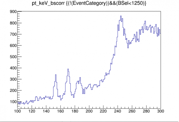
We will fit the two lines to Gaussians. Note that the 18keV line is sort of a double line as seen in this more detailed plot from the Run 68 calibration:

So it's best to avoid the left shoulder when fitting that peak.
h4pt->Fit("gaus","","",149,157)
// result:
// 2  Mean         1.53030e+02   9.79995e-02  -6.69271e-06   1.77932e-04
h4pt->Fit("gaus","","",169,176)
// result:
// 2  Mean         1.70756e+02   2.74208e-01   1.07517e-04   7.55118e-05

We see that the 13.95 keVee and 17.74 keVee lines in this -84V data show up at 153.0 keVt and 170.8 keVt.
Step 2: Fit the calibration lines to a calibration function
We use the same basic idea for the calibration here as was done for Run 68, though you will see there are some differences. The similarities are summarized here:
- The function is constructed to go through (0,0) exactly - that is, zero amplitude is assumed to be equivalent to zero energy. (Note that there's a known OF bias at very low energy, near the noise, that makes this not strictly true, but since practically our analysis threshold is several sigma above the noise wall we can ignore this.)
- The function reduces to being simply linear as energy approaches zero
- The function has only two parameters, so using the 14 and 18 keV calibration points it is an exact fit.
This produces a calibration meant to approximately represent reality at low energies by incorporating in as simple a way possible saturation effects as seen in the two lowest calibration lines. The important portion of the calibration is the nearly-linear part at low energies - we are attempting to get this linear factor as closely as we can. =
In Run 68 the form of the calibration function for high-voltage data was a quadratic constrained to (0,0). But the detector used in Run 76 (S104) has stronger saturation behavior - in particular pulse-widening kicks in at much lower amplitudes. In Run 76 the quadratic form is appropriate for 0-Volt data. But for HV data the quadratic fails - it gives nonsensical results, negative energies at the lowest amplitudes. That's because the saturation effects are much stronger at 14 and 18 keVee for S104 at high bias. Instead I've used this form:
E_cal = c * E_raw / (a - E_raw)
This satisfies the three features enumerated above, with two parameters here called c and a. a serves as a sort of complete-saturation point, which approximates the actual situation: above a certain energy all amplitudes wind up being about the same, i.e. completely saturated. (The actual value is probably not very meaningful… in all cases these fits are only expected to be good up to 18keV or a little more. Above that saturation effects get more and more complicated and more parameters would surely be needed.)
The code below shows how to extract the two parameters from the fit values:
float x1,x2,y1,y2;
x1=153.030; x2=170.756; y1=13.95; y2=17.74;
float c = y1*y2*(x2-x1)/(x1*y2-x2*y1) // (float) 13.1849f
float a = x1*(c/y1+1.0) // (float) 297.667f
We use these values to construct aliases for pt_keVee, electron-equivalent energy (here “pt” refers to the total of all channels). We also do it for the fixed-time OF so we can calculate the noise width.
z[4]->SetAlias("pt_keVee","13.1849*pt_keV_bscorr/(297.667-pt_keV_bscorr)")
z[4]->SetAlias("pt0_keVee","13.1849*pt0_keV_bscorr/(297.667-pt0_keV_bscorr)")
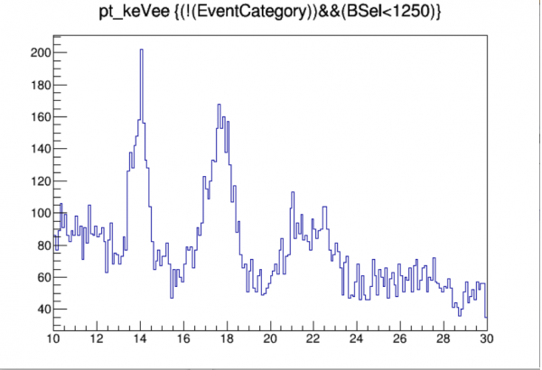
Finally you can make a histogram showing that the calibration peaks show up where they should:
z[4]->Draw("pt_keVee>>h4keVee(200,10,30)",!crand+cbs)
Step 3: some diagnostics (NTL gain, noise width)
The calibration is finished but we are now in a position to check a couple of interesting detector properties. First, we can check whether the apparent NTL gain agrees with expectations. Since the input to the calibration function is the total phonon energy (as determined from 0-Volt data), the empirical gain at low energies is just a/c, and the expected NTL gain is of course 1.+HV/3.8 (where 3.8 eV is the mean energy to produce one pair in Si).
float g_NTL_empirical = a/c        // (float) 22.5763f
float g_NTL_expected = 1.+84/3.8   // (float) 23.1053f
This is remarkably good agreement! The empirical gain is less than 3% smaller than the expected gain.
We can also check the noise width by plotting the fixed-time calibrated OF energy for randoms:
z[4]->Draw("pt0_keVee>>h4n(200,-0.1,0.1)",crand+cbs)
h4n->Fit("gaus")
// result:
//EXT PARAMETER                                   STEP         FIRST
//NO.   NAME      VALUE            ERROR          SIZE      DERIVATIVE
// 3  Sigma        9.68071e-03   1.54322e-04   2.33469e-05   9.02802e-02

The noise width comes out to 9.7 eVee. Pretty good.
Example of energy calibration with a period of NaI-coincident data
Results for periods of NaI-coincident data
| Aug 30-31 | ||
|---|---|---|
| Sep 9-10, -21V | ||
| Sep 10, -4V | ||
| Sep 12-13, -67V | ||
| Sep 13-14, +98V | ||
| Sep 16-17 | Example period | Results |
| Sep 19-21 | ||
| Sep 24 | ||
| Sep 25, -21V | ||
| Sep 25,-82V |