Table of Contents
Run 76 Summary
Main Analysis Portal
Run preparation
S104 detector
Side1pF appeared to be open in Run75. Need to investigate and try to repair this. Likely a wirebond problem since this channel was the most difficult to bond: I attempted a hopscotch, creating a spare bond pad by surgically disconnecting a stadium and repurposing it as an intermediate bond site between the DIB and one of the channel bond pads.
Thermometry
We used the Goldman thermometer for the first time in Run 75, along with the old Tower thermometer. The Goldman readings looked good - the Tower thermometer was pretty erratic and always read high. The Goldman thermometer used rerouted stripline wires, while the Tower thermometer used the standard thermometer wires that route up through the center of the fridge. There are two possibilities for the problem with the Tower thermometer:
- the Tower thermometer (or the wires connected to it) is bad
- the thermometer wires in the fridge are bad. The notion here is that maybe some insulation is partially worn away and there's a weak (high-resistance) short, essentially creating a large resistance in parallel with the thermometer. This may not be noticeable at high temperatures when the thermometer resistance is low but could become noticeable at low temperatures when the thermometer resistance is high.
If possibility #1 is correct, the thing to do for Run 76 is to use the Goldman thermometer with the fridge wiring (because with the 2D source mover we probably don't have enough stripline wires to spare, see below).
To test possibility #2 we can try measuring resistances between the thermometer wires in nS after the Tower thermometer is disconnected. If we see leakage of the right order of magnitude then we may want to try to repair these wires, which would mean disassembling more of the fridge than we usually do. (The other alternatives are to 1) reduce the wiring needs by skipping the piezo on the 2D source mover 2) build a second set of diverter board to use a second stripline for accessory wiring 3) use other unneeded wires apart from the redundant phonon returns, such as charge-related wires.)
Update
Tests of the fridge thermometer wiring at RT with no thermometer connected show no shorts. The plan is to connect the Goldman thermometer to the fridge wiring and not use the Tower thermometer.
2D Source Mover
The 2D source mover requires 8 wires for the two motors. If we want the piezo for recalibration purposes that's 2 more wires, a total of 10.
One stripline has 13 spare wires (as a rule). If we use 10 wires for the source mover we wouldn't have 4 left for a thermometer.
On the other hand there really are more spare wires available: charge-related wires are not needed. On all but one DIB, LED wires are not needed.
Update
The plan is to connect only the motor wires and the piezo wires as stripline accessories. No stripline wires will be used for thermometry - rather the Goldman thermometer will be connected to the fridge thermometer wires and the Tower thermometer will not be used.
Run Setup
Accessory wiring
| Run 76 accessory wiring | ||||||||||||||||
|---|---|---|---|---|---|---|---|---|---|---|---|---|---|---|---|---|
| accessory | Motor Y1 | Motor Y2 | Motor Y3 | Motor Y4 | Motor X1 | Motor X2 | Motor X3 | Motor X4 | Piezo1 | Piezo2 | ||||||
| acc wire | SL Yconnector | SL Xconnector | purple | purple | ||||||||||||
| Tower F4 | 1 | 2 | 3 | 4 | 5 | 6 | 7 | 8 | 9 | 10 | 11 | 12 | 13 | 14 | 15 | 16 |
| interposer conns | brn | w brn | org | w org | blu | w blu | grn | blk | blk | pur | pur | |||||
| no soc | no soc | no soc | no soc | no soc | no soc | no soc | no soc | no soc | ||||||||
| stripline | 49 | 50 | 8 | 9 | 11 | 12 | 13 | 45 | 2 | 46 | ||||||
| label | pBr3 | pBr4 | pCr3 | pCr4 | pAr3 | pAr4 | pAr5 | pDr3 | pAr1 | pDr4 | ||||||
| STRIPLINE ## | ||||||||||||||||
| CABLE # | ||||||||||||||||
| stripline D50 | 36 | 18 | 8 | 23 | 4 | 19 | 1 | 41 | 17 | 40 | ||||||
| DCRC/diverter Dsub | 48 | 33 | 10 | 28 | 14 | 32 | 17 | 43 | 1 | 44 | ||||||
| Dsub diverter board | U09-2 | U10-3 | U06-3 | U07-3 | U08-4 | U09-1 | U10-4 | U06-4 | U01-4 | U07-5 | ||||||
| Run75 Warm-side Accessory Wires: Motor coil (MC), endstop (ES), Goldman thermometer (GT) | ||||||||||||||||
| diverter board wires | MC Orange | MC Brown | MC Red | MC Yellow | GT Black | ES White Blue | ES Green | GT White | GT Red | GT Green | ? | |||||
Setup
| Run 76 Channel Map | |||||
|---|---|---|---|---|---|
| Tower | Cable | DCRC(2sided) | Label | HV output, Side1-readout | HV output, Side2-readout |
| Face5pA | Cable 2 (includes LEDs and accessories) HV CONN1 | DCRC3 | Side1pE | HV1 pA | - |
| Face5pB | Side1pB | HV1 pB | - | ||
| Face5pC | Side1pD | HV1 pC | - | ||
| Face5pD | Side2pE | - | HV2 pD | ||
| Face3pA | Cable 1 HV CONN2 | DCRC1 | Side2pC | - | HV2 pA |
| Face3pB | Side2pF | - | HV2 pB | ||
| Face3pC | Side1pC | HV2 pC | - | ||
| Face3pD | Side1pF | HV2 pD | - | ||
| Face2pA | Cable 3 HV CONN3 | DCRC4 | Side2pB | - | HV1 pA |
| Face2pB | Side2pA | - | HV1 pB | ||
| Face2pC | Side1pA | HV2 pB | - | ||
| Face2pD | Side2pD | - | HV1 pD | ||
Source mover tests
2-sided 0V
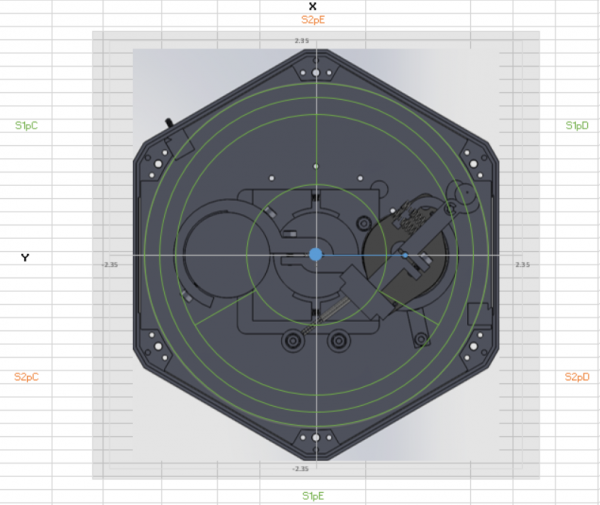
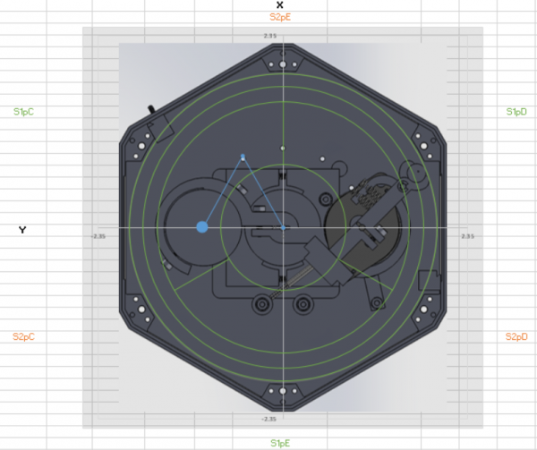
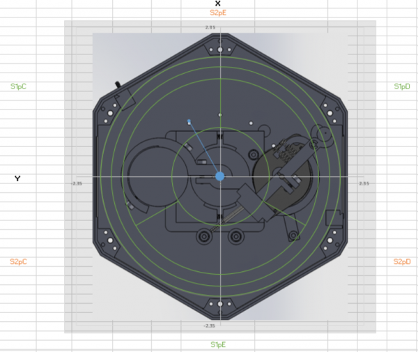
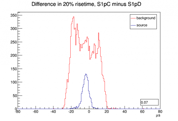
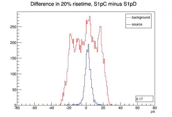
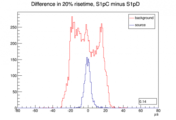
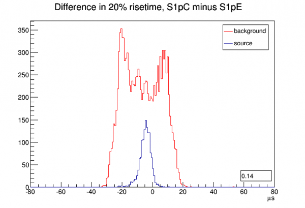
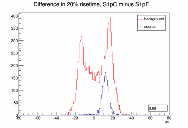
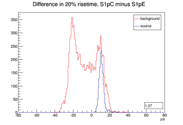
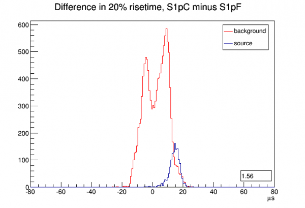
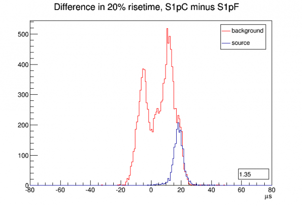
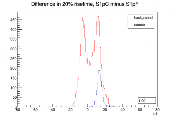
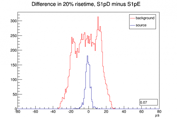
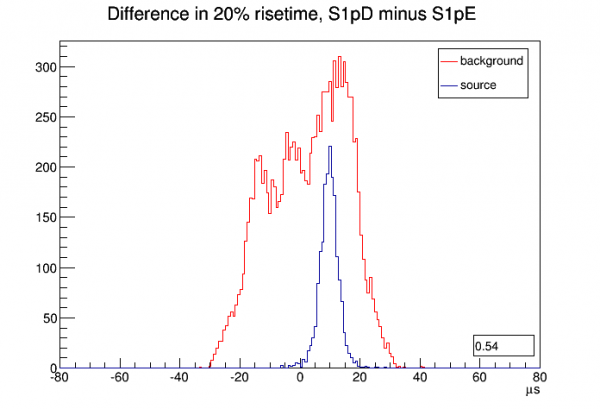
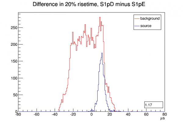
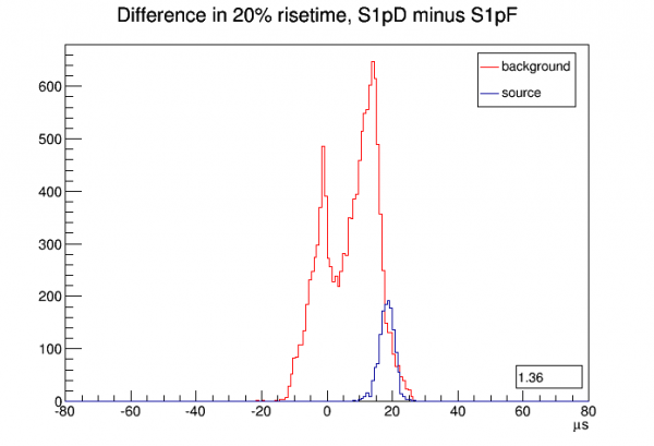
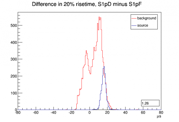
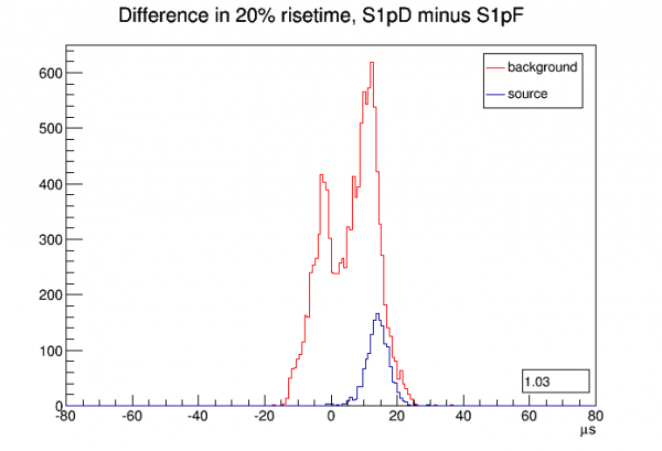
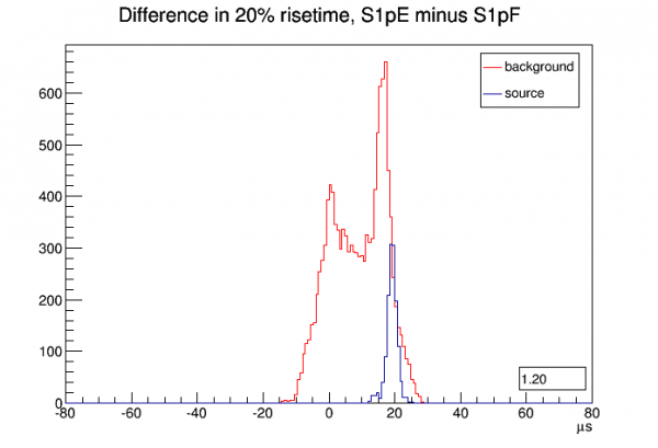
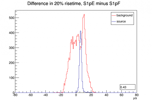
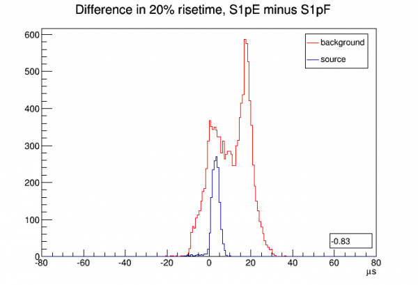
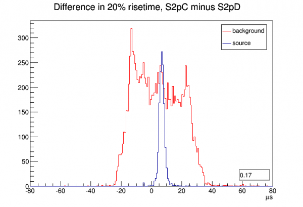
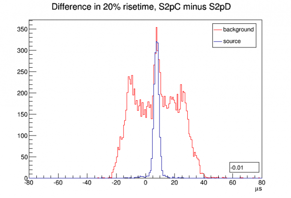
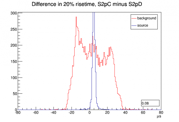
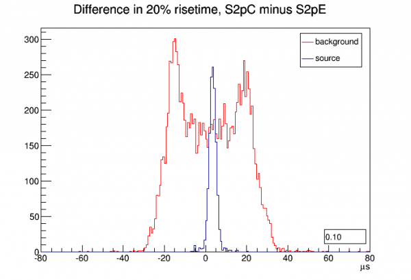
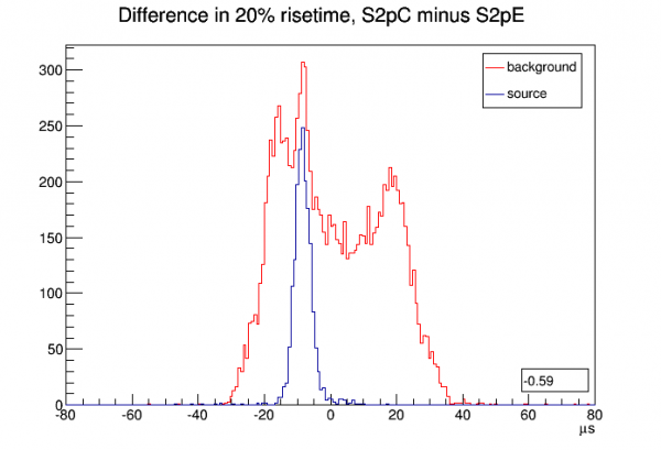
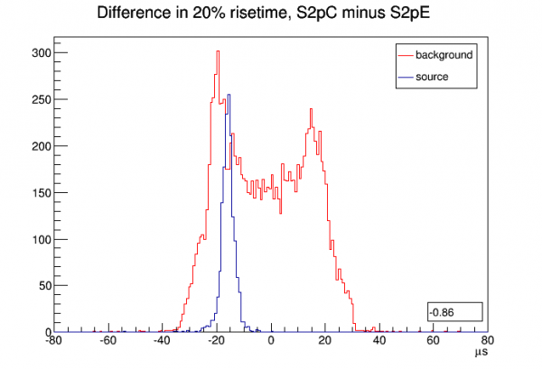
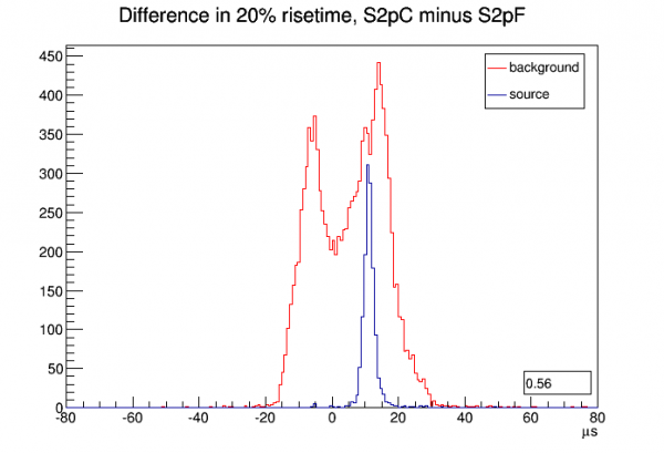
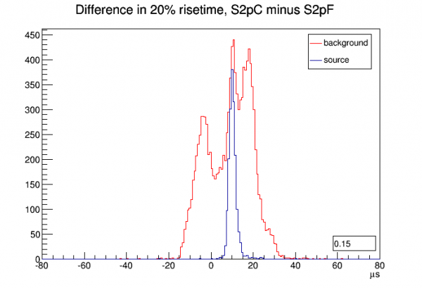
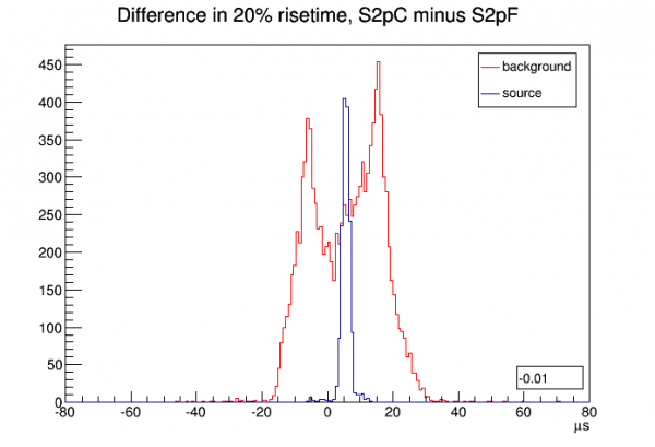
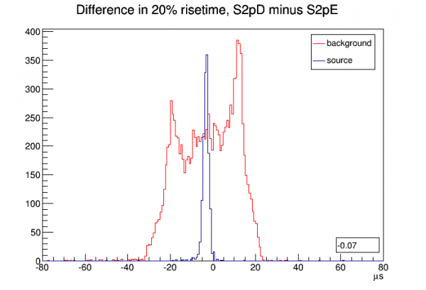
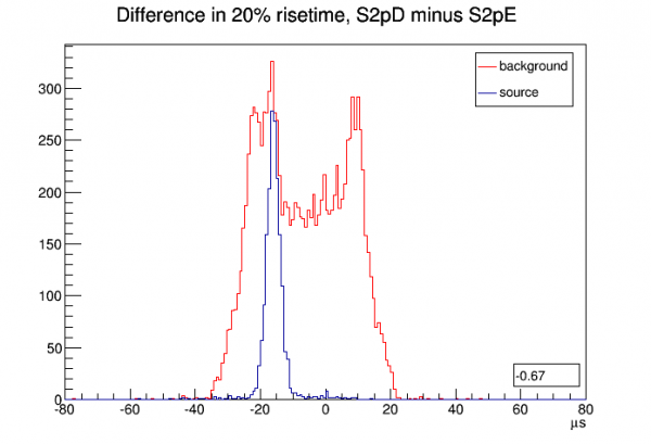
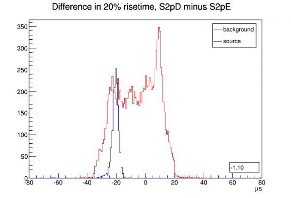
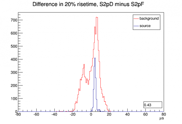
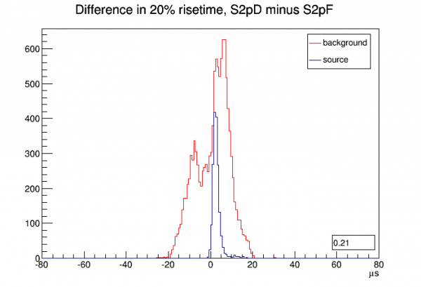
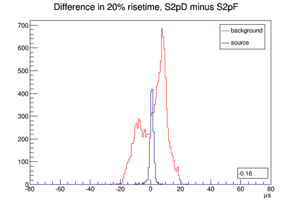
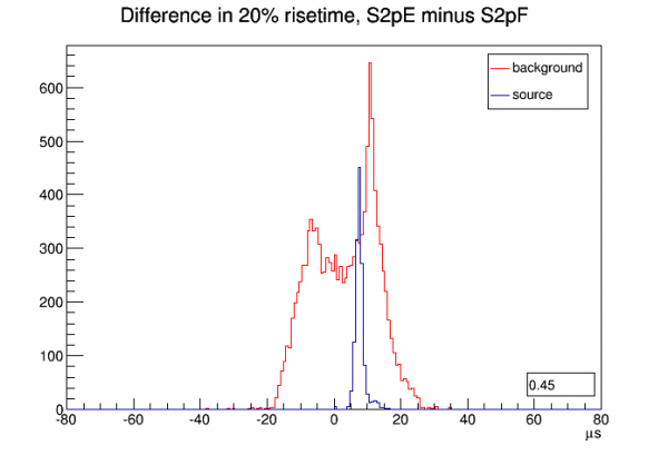
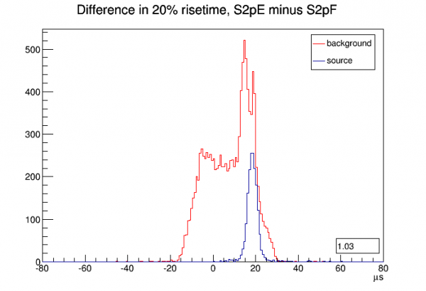
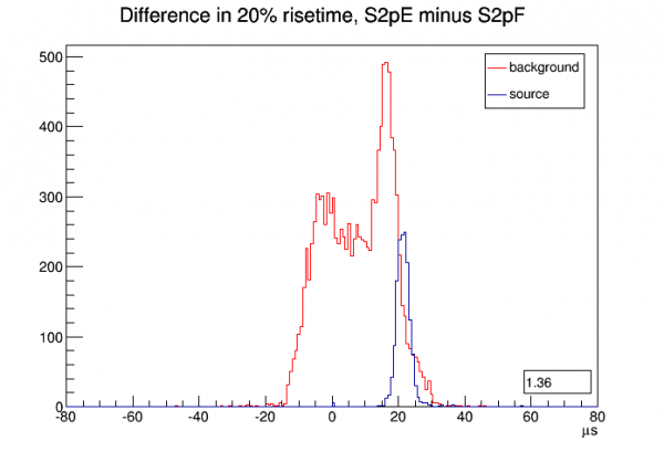
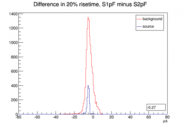
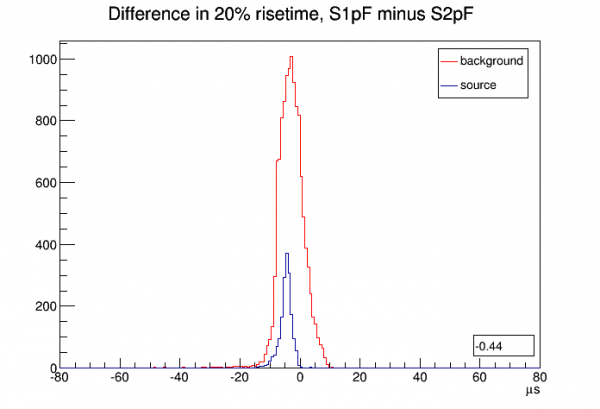
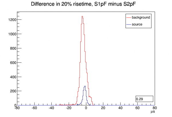
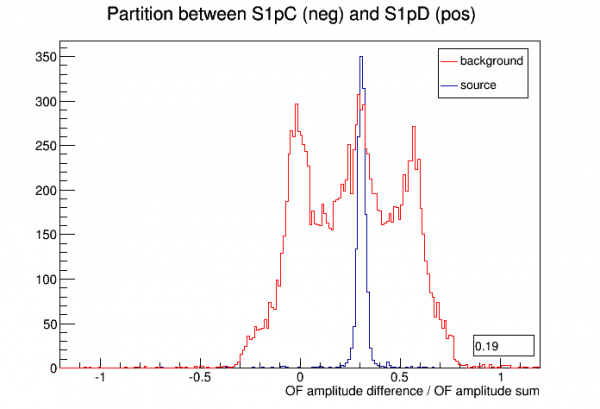
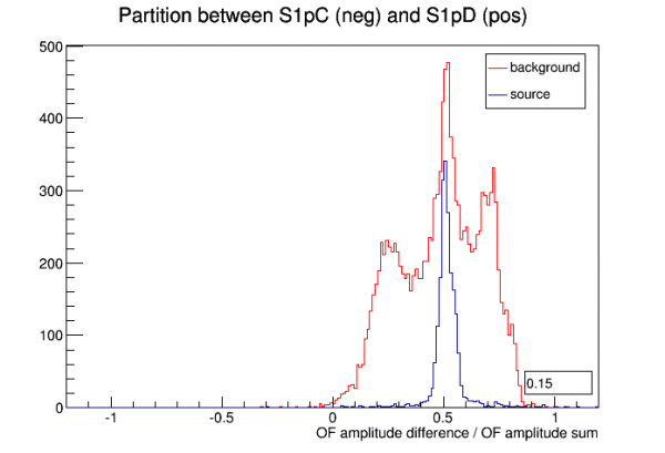
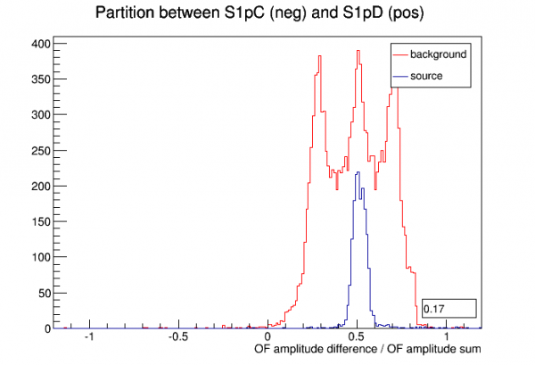
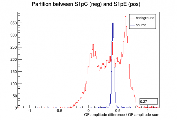
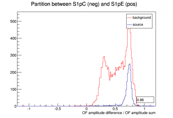
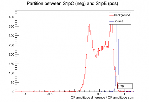
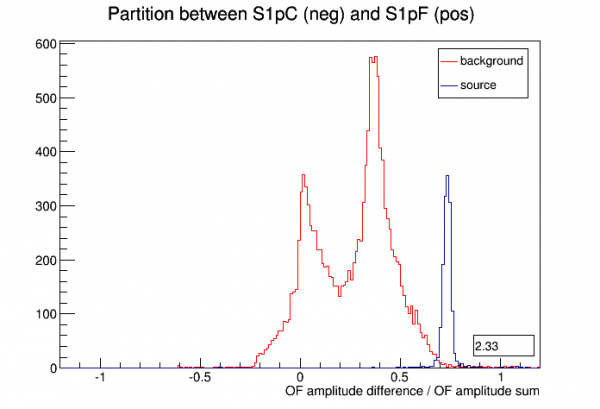
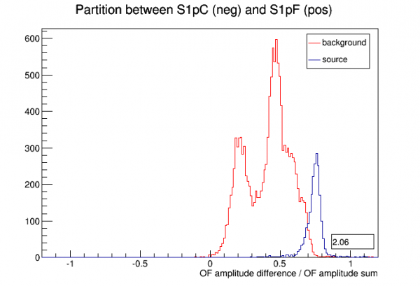
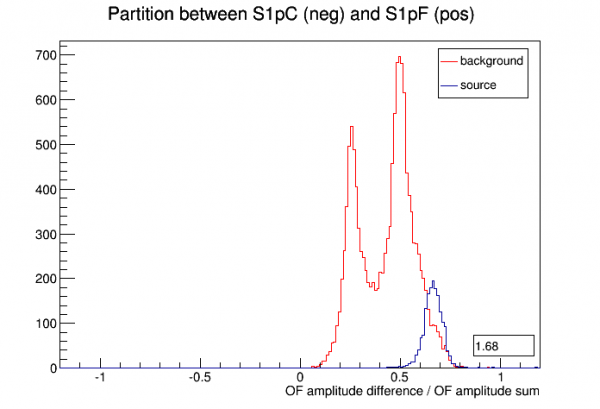
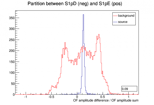
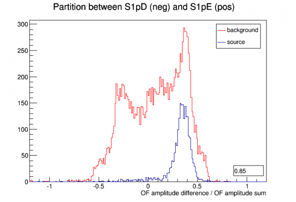
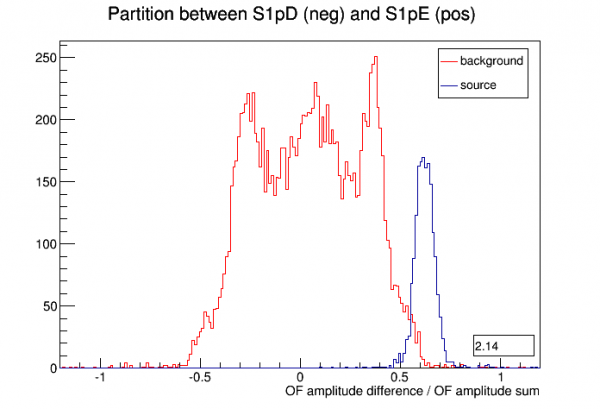
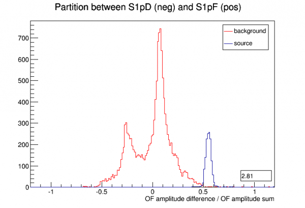
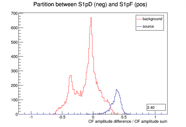
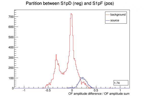
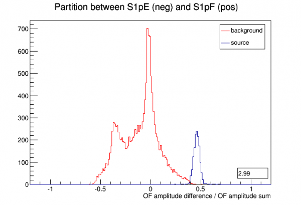
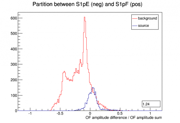
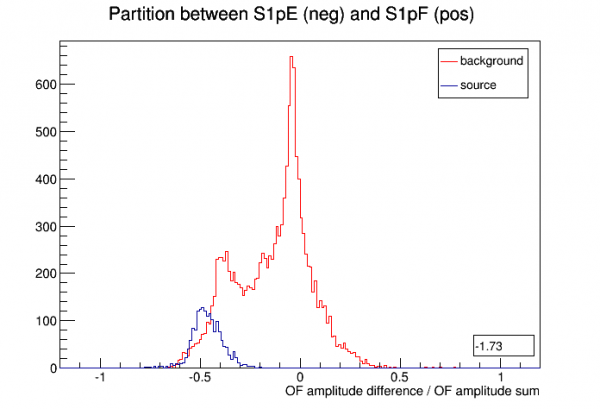
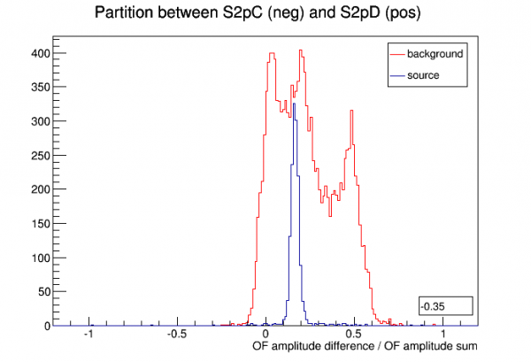
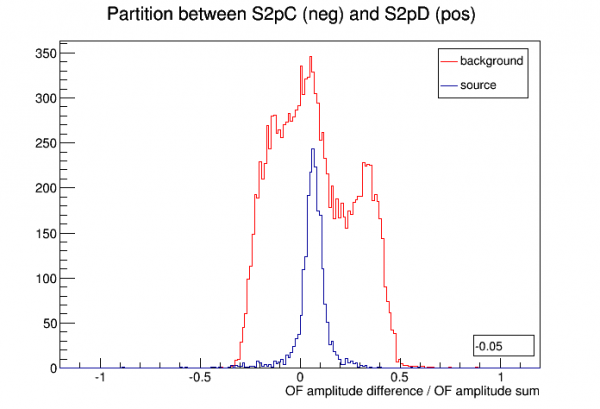
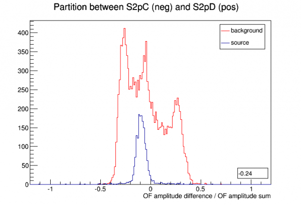
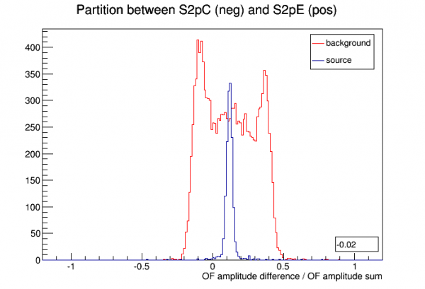
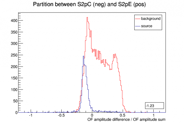
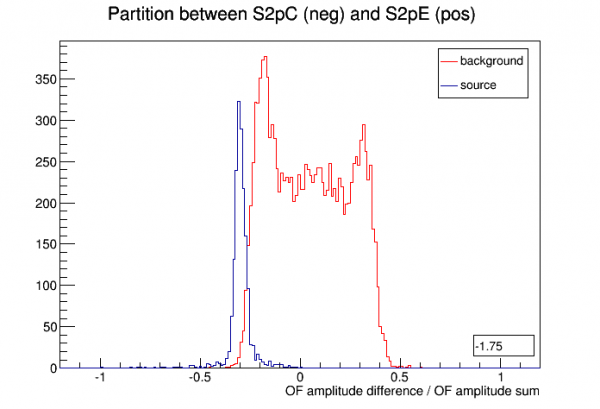
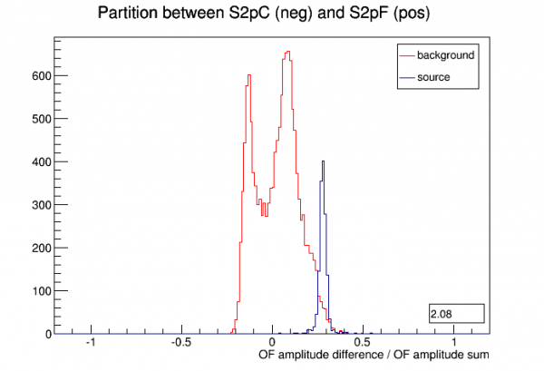
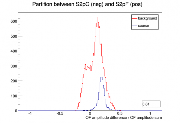
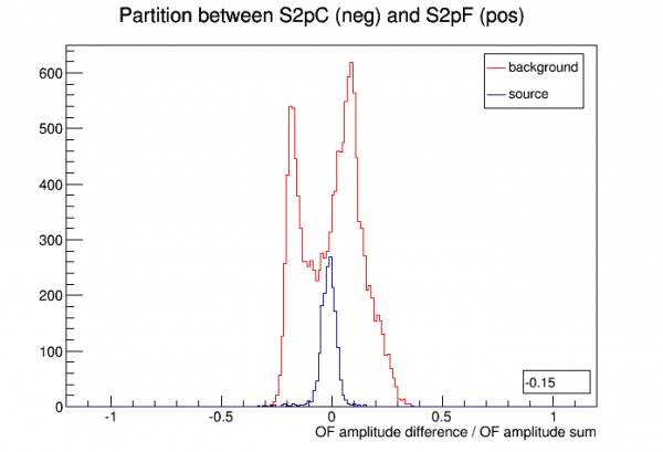
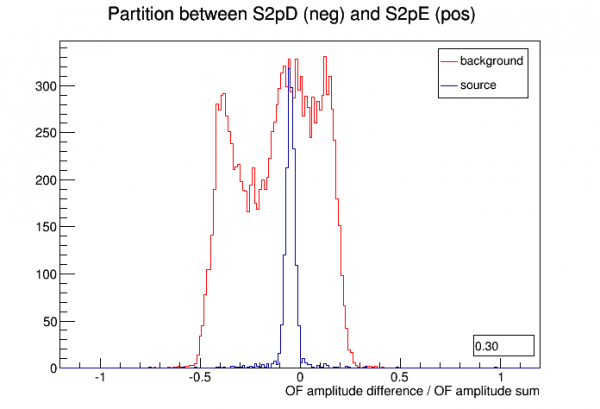
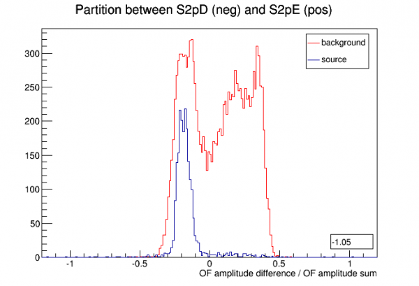
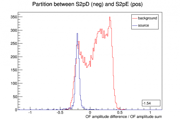
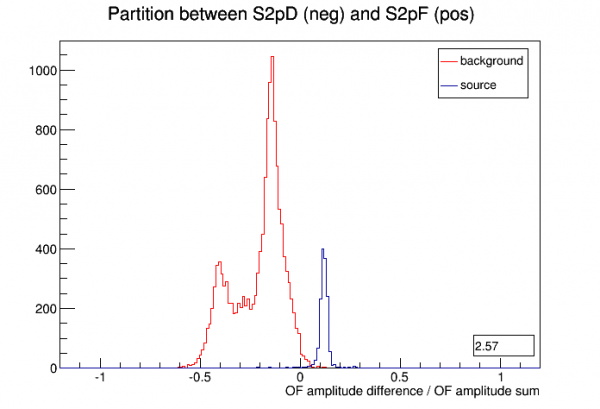
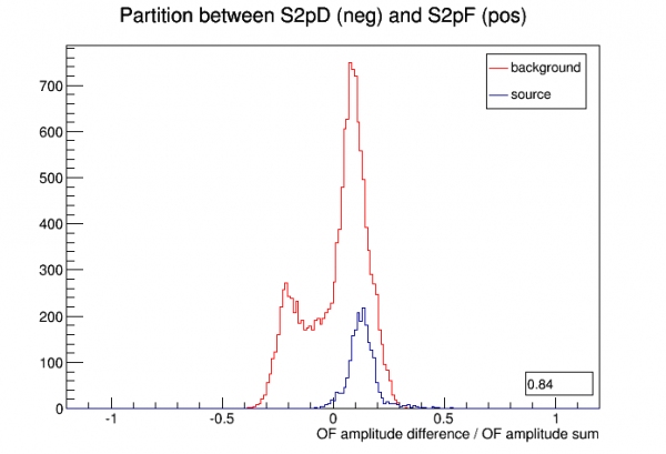
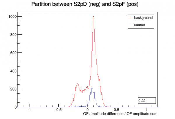
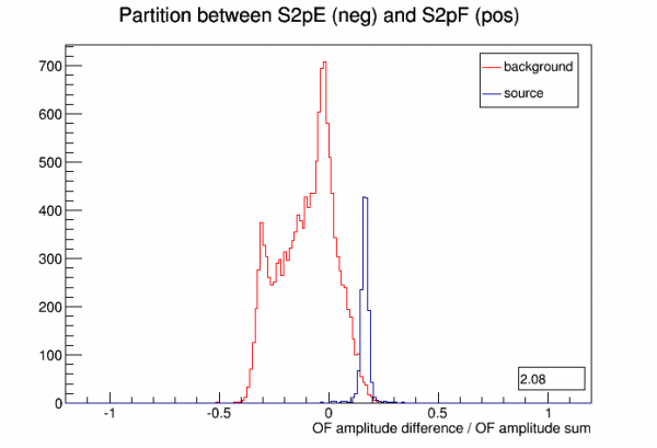
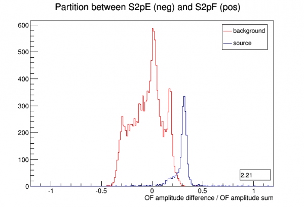
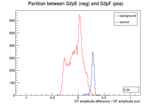
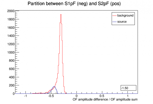
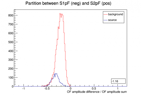
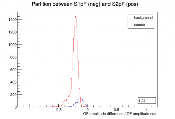
The number in the lower right in the plots below is (mean_of_source_distribution - mean_of_background_distribution)/stdev_of_background_distribution
| First Position | Second Position | Third Position |
|---|---|---|
 |  |  |
| Delays | ||
 |  |  |
 |  |  |
 |  |  |
 |  |  |
 |  |  |
 |  |  |
 |  |  |
 |  |  |
 |  |  |
 |  |  |
 |  |  |
 |  |  |
 |  |  |
| Partitions | ||
 |  |  |
 |  |  |
 |  |  |
 |  |  |
 |  |  |
 |  |  |
 |  |  |
 |  |  |
 |  |  |
 |  |  |
 |  |  |
 |  |  |
 |  |  |
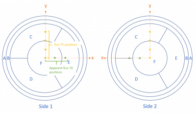
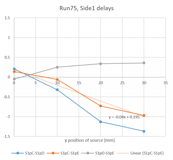
Link: Similar plots from Run75 with 4 known positions using the 1-D source mover.
 |  |
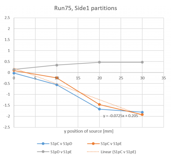 | 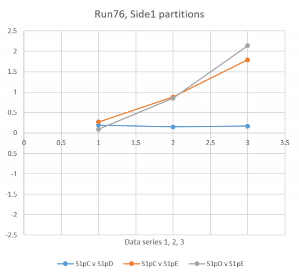 |
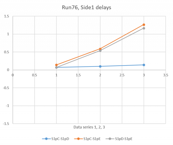
In Run 75 the source was moved toward Side1pC and sort of parallel to Side1pE. In Run 76 the source is apparently moving toward Side1pE and therefore sort of parallel to Side1pC and Side1pD. So it makes sense to compare these trends. Doing so implies that the second position in Run 76 is at x=11.5 mm judging from delay, x=9.4 mm judging from partition. The third position in Run 76 is at x=27.9 mm judging from delay, x=24.6 mm judging from partition.
Plots not shown but I also tried to get a pure radius quantity with delay between Side2pA and Side2pF. Comparing Run75 and Run76 implies the following Run76 positions: Position 1/2/3 → r = 0/19/21 mm.
- first series
- 1B (DCRC3pB) shift at 220e3 (~6 samples up)
- 2C (DCRC1pA) shift at 60e3 (~7 samples up)
- 2F (DCRC1pB) shift at 160e3 (~6 samples up)
- second series
- 1C (DCRC1pC) shift at 120e3 (~7 samples up)
- 2F (DCRC1pB) shift at 105e3 (~7 samples up)
- 2C (DCRC1pA) shift at 55e3 (~6 samples up)
- third series
- 2C (DCRC1pC) shift at 90e3 (~7 samples up)
Identifying r of source statistically
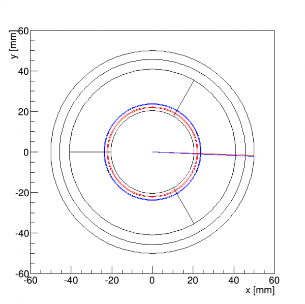
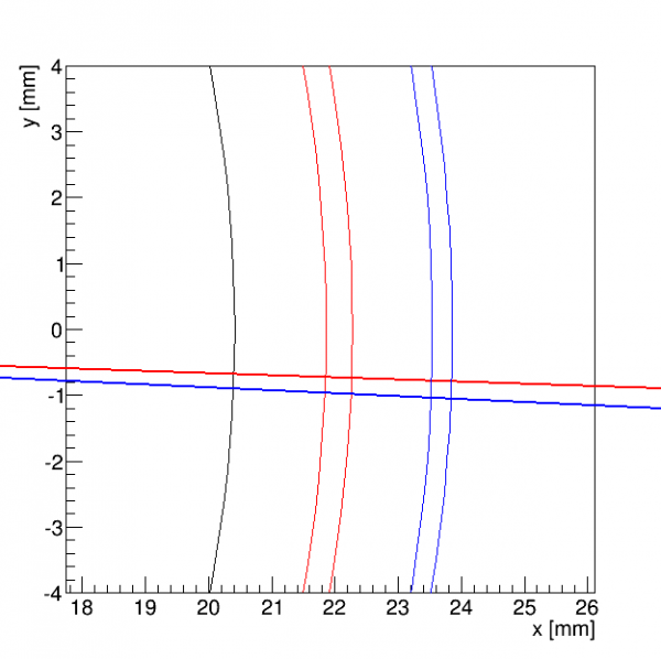
Here I show another method for identifying the third source position. Phi based on delay in the three inner-ring channels (pC,pD,pE) seems to be a reliable way to get the phi angle of the source, at least for the position it's currently at. This uses Side2 0V data from June - could extend it to 2-sided data.
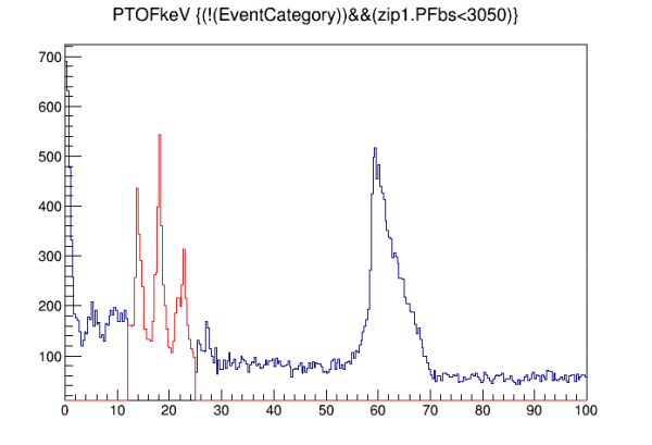
First we use the phi_del distribution to identify Am-241 events. Then we plot pFtime-pAtime both for Am events and background events. Assume 1) that background events are uniformly distributed and 2) that pFtime-pAtime increases with radius, at least from r=0 to the radius in question (if it becomes degenerate at high radius this method will still work). Also we assume 3) symmetric behavior in the detector, though we've seen evidence that the pFtime-pAtime quantity has a dip in a certain range of phi.
We find the central value of phi_del for the Am distribution, call this rdel_Am. Then we integrate the background distribution from its smallest value to rdel_Am and compare that to the integral of the entire distribution. Assume that ratio is proportional to the ratio of the areas of the circle defined by r_Am to the area of the detector, and use that to find r_Am.
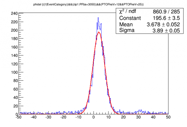 |  |
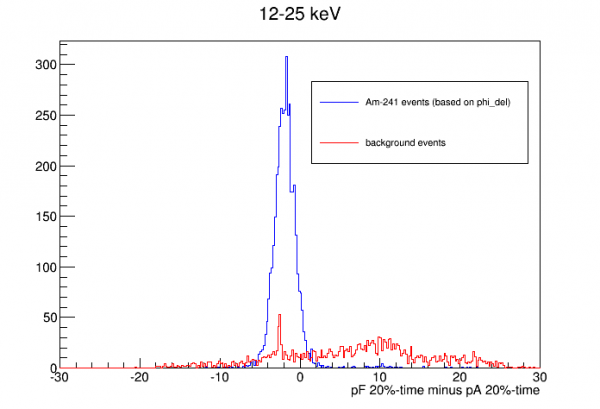
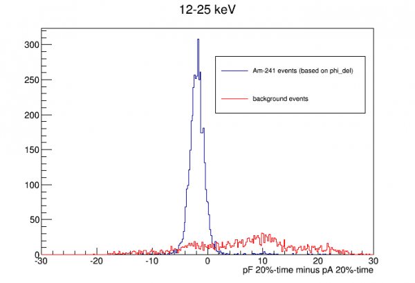
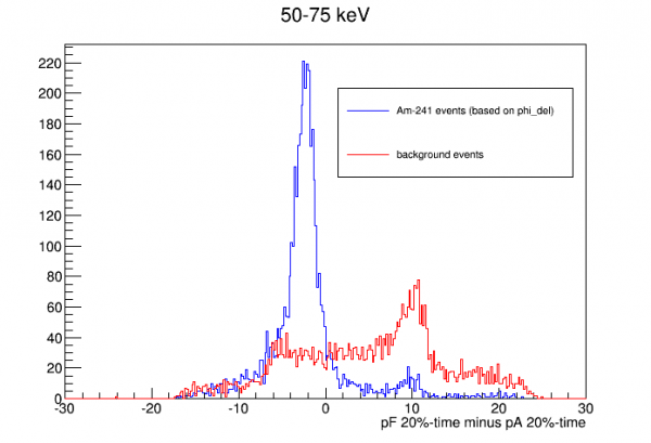
phi of source = -1.89251 +/- 0.0195322 degrees
60keV: phi of source = -2.52222 +/- 0.0317306 degrees
r of source = 22.0671 +/- 0.206736 mm
60keV: r of source = 23.7012 +/- 0.158923 mm
 |  |
Muons in NaI array
A calculation of cosmic-ray muons in the NaI array was done to inform trigger strategies to reduce the muon background rate.
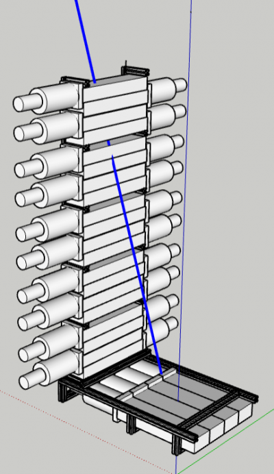
The muon flux at sea level is taken to be

where C = 0.0083 /cm2/SR/s. This implies a total of 0.0130 muons/cm2/s through a horizontal surface (1 per cm2 in 77 seconds) and 1/4 as much through a vertical surface.
In NaI a minimum-ionizing muon deposits 4.785 MeV/cm. The paddles are 5.7 cm thick (ignoring the thickness of the metal casing) so the minimum energy deposited by a through-going muon is 27.27 MeV. By through-going I mean a muon that enters the top surface and exits the bottom surface of the detector. Clipping muons in contrast are those that either enter or exit through one of the vertical sides - these can deposit less than 27.27 MeV.
Muon calculation #1: vertical array only, no gaps included
For ease of coding the first calculation considers only the vertical stack of 20 detector paddles and ignores the gaps between each set of 4.
The code treats the stack of 20 detectors as a single unit. For each of the 5 surfaces which a muon could enter, the code loops through two position coordinates and two angles. The default spacings are 1 cm and 1 degree. For each set of coordinates and angles the differential rate is calculated, and the rate, initial and final z of the track, and angle theta with the vertical are recorded in a Root tree. These four quantities are sufficient to determine which detectors are hit and how much energy is deposited in each.
In a separate incident of the code it calculates the muon rate for different categories of tracks:
| Muons per second which: | ||||||||
|---|---|---|---|---|---|---|---|---|
| Enter a wide face and exit… | Enter a narrow face and exit… | Enter the top and exit… | ||||||
| a narrow face | the opp. face | the bottom | a wide face | the opp. face | the bottom | a narrow face | a wide face | the bottom |
| 5.70 | 18.62 | 4.02 | 5.80 | 0.54 | 1.20 | 1.19 | 4.08 | 0.10 |
| 28.33 | 7.54 | 5.37 | ||||||
| 41.25 | ||||||||
These values are all a little smaller than calculations based on the area of the surfaces, likely due to errors introduced by the rather rough binning.
(note to self: if loop doesn't quite span the full range, on the last one I should expand the differential element and increase the rate accordingly.)
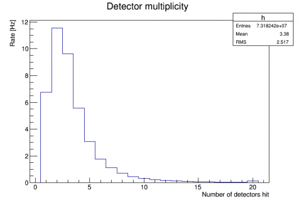
The figure above shows the rate for each possible number of detectors hit. The highest rate is for muons that hit two paddles.
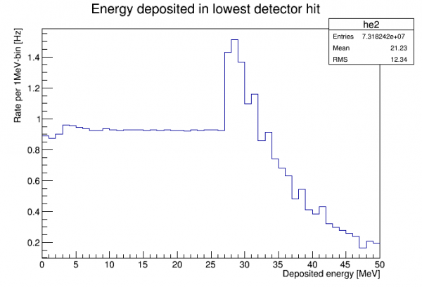
The figure above shows the energy distribution in the lowest detector hit. All energies below 27.27 MeV represent clipping muons. (The maximum possible energy in a single detector is 201.25 MeV - this plot cuts off at 50 MeV.)
We can consider the effect of a trigger that requires that every paddle has less than 27.27 MeV. Note that this automatically eliminates events which hit more than 2 detectors, since these necessarily include intermediate detectors in the path which experience a through-going muon. So a cut of this kind makes a multiplicity cut unnecessary. To determine the rate of muons that pass such a cut we sum the rates for cases in which the multiplicity is less than 3 and the energy in each of the remaining detectors is less than 27.27 MeV. The result is:
Rate of muons in which each detector has less than 27.27 MeV: 2.03 Hz
Another cut strategy would be to use the top and bottom detectors as vetos:
Rate of muons that don't hit the top or bottom detectors: 25.33 Hz
We could also combine these two criteria, though the result is not much better than the first case above:
Rate of muons in which each detector has less than 27.27 MeV and neither the top nor bottom detector is hit: 1.81 Hz
Another trigger strategy would be to require that at least one detector has energy below 27.27 MeV (and above some lower threshold). The rate of muons that would be accepted by this criterion is:
Rate of muons such that no detector has energy >= 27.27 MeV: 32.04 Hz
Muon calculation #2: horizontal array only
The second calculation considers only the horizontal row of 3 detector paddles situation under the cryostat. (Note: the figure above showing 4 detectors in a row is not accurate.) The code is similar to that used for the vertical stack.
Total muon rate in horizontal row: 18.75 Hz.
This is quite close to a calculation based on the area of the surfaces.
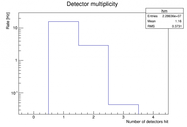
The figure above shows the rate for each possible number of detectors hit. 84% of muons hit only one detector.
Rate of muons in horizontal row in which each detector has less than 27.27 MeV: 4.82 Hz. This is more than twice what the same criterion yields for the 20-detector vertical stack.
Combining vertical and horizontal parts
It's a bit more work to account for muons that hit both the vertical and horizontal parts of the array. The simplest estimate is to simply add the calculated rates from the two pieces. This will double-count some muons so these will be overestimated.
Assuming no muons hit both the vertical and horizontal parts of the array:
- Total muon rate in full array: 60.00 Hz
- Total rate in which each detector has less than 27.27 MeV: 6.85 Hz
Comparing muon calculation to data
Using spectra taken in the lab with the NaI detectors, we can perform the same sort of muon calculation for a single detector and compare both the spectrum and the rate to actual data.
Data: DataF_CH0_DT5751_626_NaI-Array-Det1-1121V-Bknd-20220322-Na22.root
The data used is an Na-22 calibration taken for 100.15 seconds (real time) in Detector 1 (top of vertical stack). The muon calculation was scaled to the same time.
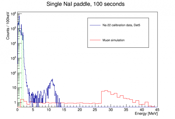
The plot above shows the full spectrum from the data. A calibration performed on the three prominent Na-22 peaks (511, 1274, 1786 keV) is quite linear. (Note: to get a good calibration you must allow for a 0-energy offset.) Also, PuBe data taken later showed good linearity up to 4.4 MeV. But there seems to be strong saturation at the muon bulge energy, minimum 27.27 MeV.
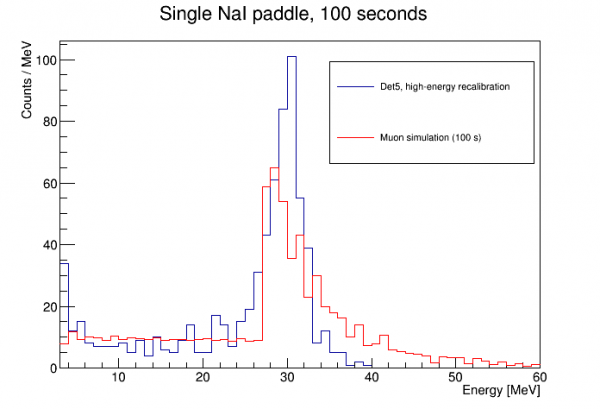
In the plot above a simple linear high-energy recalibration was done using two points: 4 MeV from the original low-energy calibration, and the muon-bulge minimum. Here the time-normalized muon calculation shows a remarkably good fit.
For both the data and the calculation I counted the total number of events between 5 and 25 MeV:
- Data: 177 events (1.78 Hz)
- Calculation: 187.9 events (1.88 Hz)
These are consistent within about one sigma.
Conclusion: The simple muon flux model used here is a good approximation of the actual high-energy spectrum seen in the NaI detectors. No additional source of high energy events is noticeable.
Noise width in HV
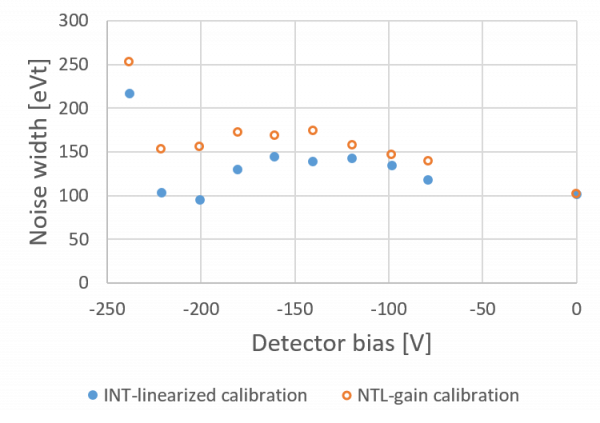
With Side2-readout and negative HV bias we've been able to resolve the 14 and 18 keV lines using pulse width. Several HV biases were studied to see which produced the lowest electron-equivalent noise.
The first calibration attempted was the same that was used in Run 75. A 0-intercept quadratic function is used to linearize PTOF with respect to PTINT up to the 14 keV line. This linearized PTOF is then calibrated to the 14 keV line.
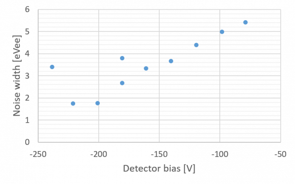
The plot above shows remarkably good noise width at bias around -200V.
Is it really this good? It depends on how good the calibration is. We are relying on the fact that PTINT remains proportional to energy up to 14keV. In fact estimates of the 2nd-order TES effects suggest that it may drift down from proportionality by as much as 15% at 14keV. Saturation effects could make the pulse integral even lower. However: if the signal amplitude is lower than expected, the calibration algorithm used would tend to make the noise width look worse. So saturation arguments would suggest that the noise width is even better than in this plot.
On the other hand the 14keV line as seen in linearized-PTOF is very wide. It's questionable whether taking the Gaussian center is very accurate.
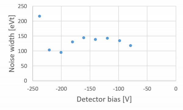
The figure above uses the calculated NTL-gain to show total-phonon-energy noise width as a function of bias. This raises some doubt since we generally expect the pT noise width to rise at least somewhat as bias increases. Here it suggests that it's actually somewhat better at high bias than at 0V. This suggests that perhaps that the noise widths are worse than what we have calculated.
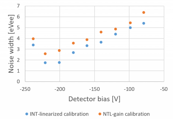
The plot above shows an alternative noise width based on an alternative calculation. Here we use the 0V PTOF calibration (at 0V both PTOF and PTINT seem very linear up to 14keV) and simply use the calculated NTL gain to adjust this calibration to the HV case.
Calibrating HV data
Initially I attempted a calibration of Side2-readout HV data similar to what was done in Run75: linearize pT-OF to pT-INT then calibrate linearly to the 14keV line. But the 14keV line is so spread out and distorted in both pT-OF and pT-INT in HV data (it only resolves well in pulse width) there's probably large systematic error.
Here I show an alternative calibration based on 0V data and calculated NTL gain.
Summary of technique
The idea is to calibrate 0V data using the 14keV line, then simply scale this calibration for HV data by calculating the NTL gain from the measured bias. (Note that HV current leakage has been very small this run, with corrections to detector bias less than 1%.)
We want the 0V 14keV calibration to be valid for HV data in the region of interest, 0-2 keV. Two corrections are applied:
- correction for baseline. We can see the expected variation in calibration peak position with phonon baseline in the 0V data. Elevated baselines generally result in lower TES gain. We correct the raw OF amplitude using the baseline. This is meant to account for multiple things: the somewhat higher baselines seen in HV data (which may be caused by parasitic power); variations in detector temperature that could affect gain; and gain reduction due to an event being on the far end of a tail of a previous event (events too close to previous events are removed by cuts).
- correction for pulse width. Since we are using a single-template OF fit, differences in pulse shape will produce systematic differences in reconstructed amplitude. As above the effect is measured using 0V data. The attenuation of the 60keV line seen when using the 14keV-based calibration, and the pulse widths of events at 14keV versus 60keV, are used to characterize this effect.
Example
Data used for this example were taken on 2022 May 10:
- 07220510_0917, 0V
- 07220510_1115, -195.6 V
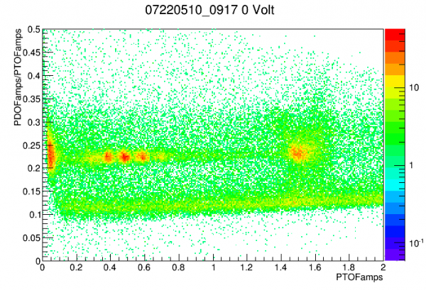 |
| In the 0V data, the peaks are clearly identifiable in pD-fraction versus pTOF. A partition cut can be defined to make them stand out better from background. |
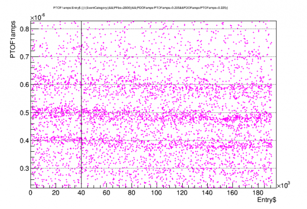 |
| For some unknown reason this data has a time dependence. A cut was made to choose only the early data. |
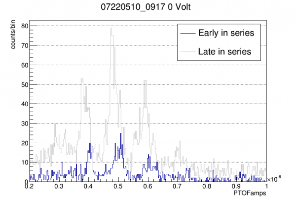 |
| Later data has significantly decreased gain. For the calibration only early data is used. |
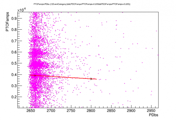 |
| Plotting amplitudes versus one of the baselines reveals the downward trend in energy. A linear fit is the basis for a correction function used both here and in HV data. |
 |
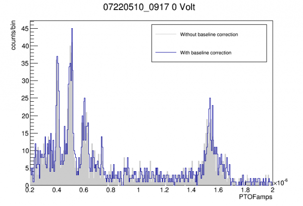 |
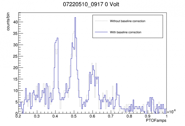
| Peaks are somewhat better resolved after baseline correction. |
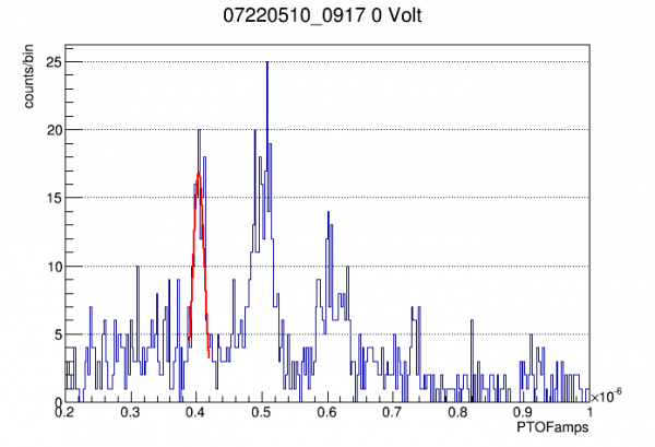 |
| The 14 keV peak is the basis for a linear calibration on baseline-corrected pTOF. |
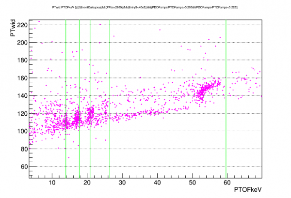 |
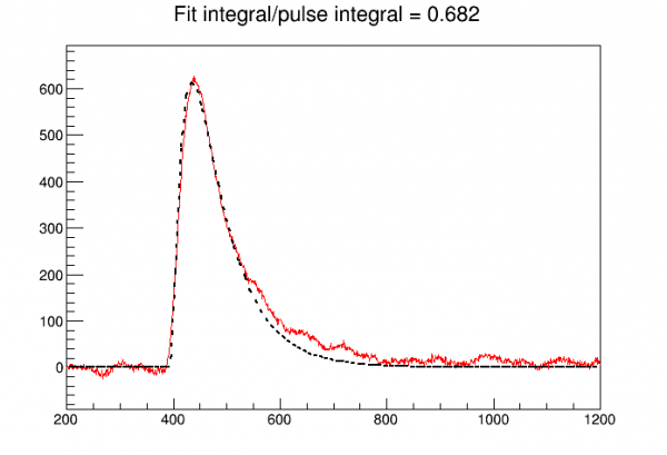
| Higher-energy peaks are wider (width is calculated as 40%-time on falling edge minus 40%-time on falling edge) and have attenuated amplitudes with respect to the linear calibration on the 14keV peak. The relative suppression and average width of the 60keV peak is used as the basis for a linear width-correction of amplitude. |
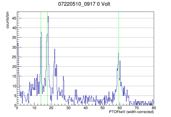 |
| Here is an example of a width-corrected spectrum in the 0-V data. |
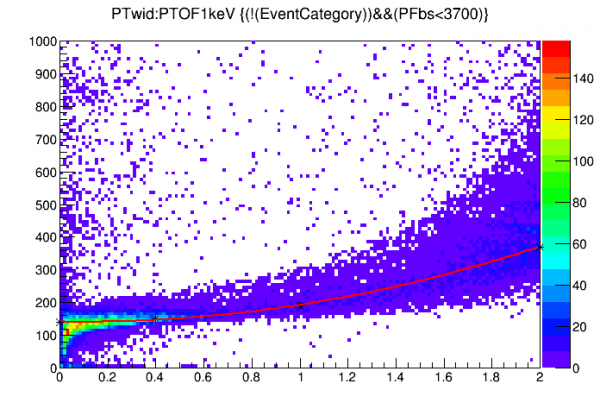 |
| In HV data, the pulse width is plotted as a function of energy from 0-2 keV. Here we have already applied the NTL-based calibration and the baseline correction. To correct for pulse width, rather than using the measured pulse width I have instead fit the pulse width to the (uncorrected) energy to instead use that function to make a correction that doesn't depend directly on each event's measured pulse width. The reason is that the walk algorithm is not particularly well-resolved; this is an attempt to retain the intrinsic resolution of the OF algorithm. (Alternatively we could correct directly to pulse width which would sacrifice resolution but allow for position-dependent width variation. |
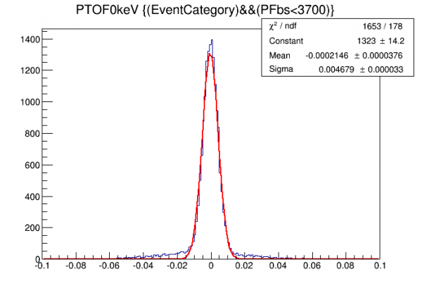 |
| Here we use the fully corrected calibration to measure noise width. It's around 50% worse than previous calculations that did not use baseline and width corrections. |
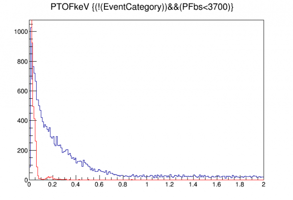 |
| A first look at the low-energy spectrum after corrections. There's a large excess at the low end. The red curve shows randoms with the same calibration applied, so that excess extends to energies well above the noise wall. Viewing pulses in that range reveals many on downward-sloping baselines. No pileup cut or tail cut has really been applied yet. |
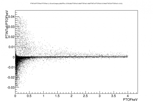 | 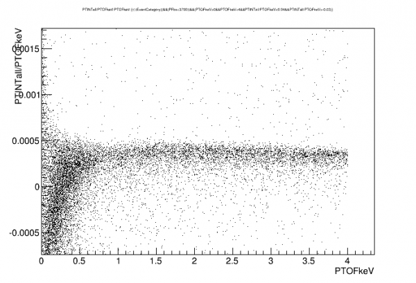 |
| One cut strategy to remove pileup and tail events is based on the ratio of INT to OF. This should form a band when plotted versus energy; pileup and tails will appear as outliers. | |
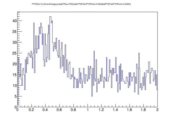 |
| A much better spectrum is seen after applying an OF-INT agreement cut. |
More on the pulse width correction
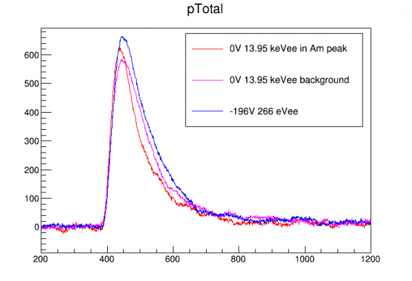
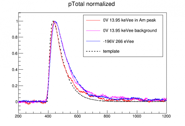
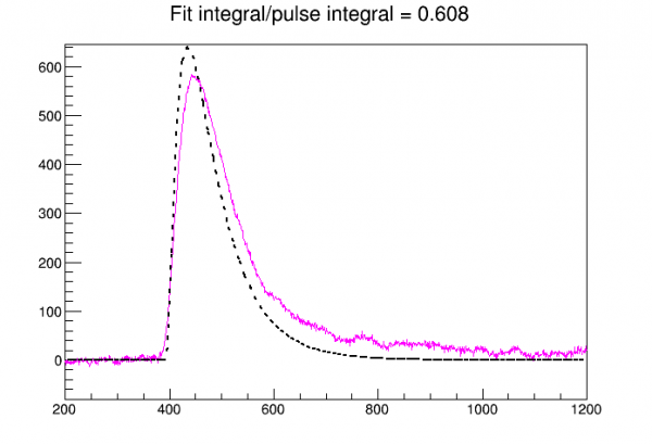
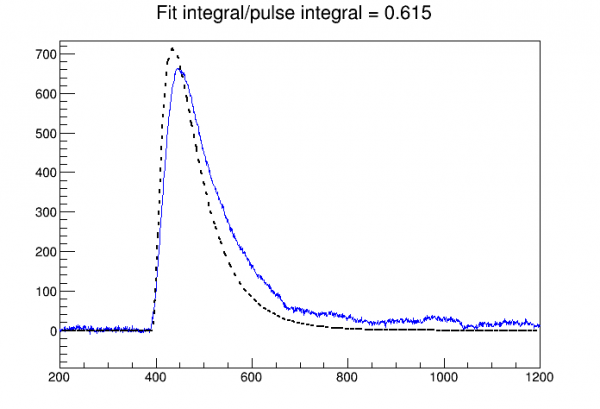
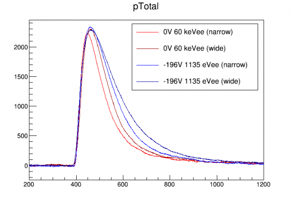
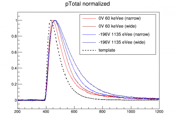
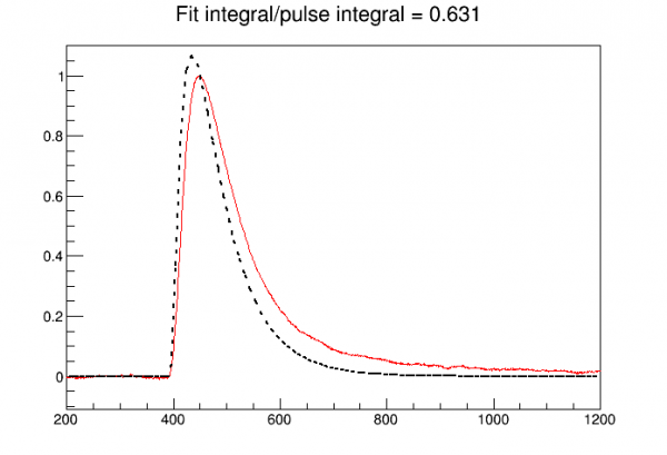
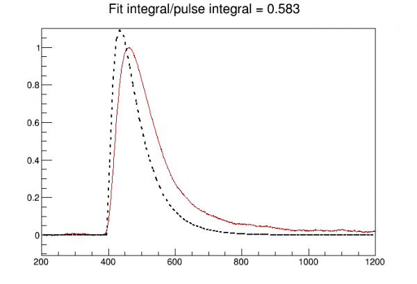
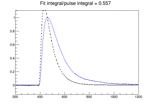
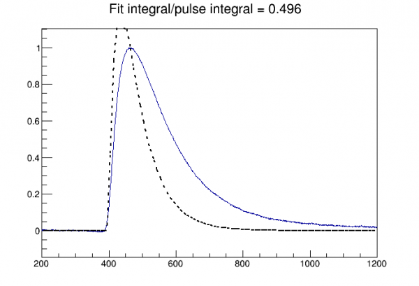
In the 0 Volt data, events in the 14 keV peak have a width of around 110 us, and events in the 60 keV peak have a width around 150 us. For events with the same total phonon energy in HV data we see wider pulses, around 140 and 210 us respectively. Two questions arise: why are the pulses wider in HV data? is the correction appropriate for these events?
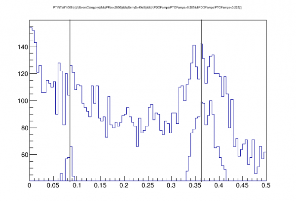 |
| We see amplitude attenuation with pulse width in OF in the 0 Volt data. If this is due to template/pulse mismatch, then we wouldn't expect to see attenuation in INT. This plot checks that. Unfortunately the 14keV peak is not resolved in INT. But we can use cuts to select the peaks in OF and apply these cuts to see the two lines in INT. The vertical superimposed lines are separated by the known 60keV/14keV ratio. This shows that there is no attenuation in INT. (In fact if anything it looks like the 14keV peak is too low with respect to the 60keV peak, maybe around 10%. Could this be some near-surface effect that cause energy loss? Not sure if I'd expect that in 0 Volt data.) |
I decided to investigate whether the position of the 14keV events might be making their pulse widths narrower than most other events at 0V.
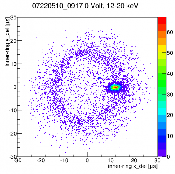 |
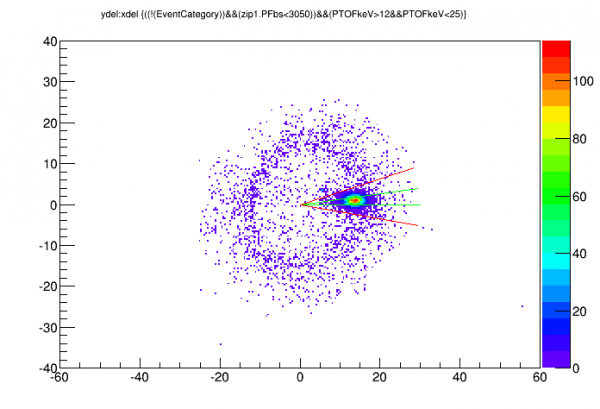
| y-delay versus x-delay (based on inner ring channels) in an energy range that includes the low-energy Am lines. Am lines are clustered at a well-defined angle on the donut. |
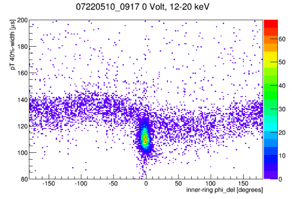 |
| Pulse width versus phi-delay (angular position of event) in the 12-20 keV range. In background events there's a curved band showing some angular dependence of pulse width. But Am events are on the lowest extreme of this band. |
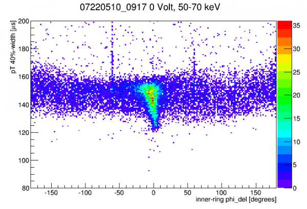 |
| Same plot as above but for the 60keV energy region. Here Am events seem to mostly follow the same pulse width band as background events, with some 60keV events extending down to lower widths. |
Conclusion: pulse width is smaller for near-surface events. Note that the readout is on the opposite side as the source. But CDMS lore tells me that near-surface events can cause faster risetimes even with readout on the opposite side, because many carriers will hit an electrode very early and lose their conduction-band energy, and the relaxation-phonons produced are faster (ballistic) than primary phonons (diffusive).
Below I copy a figure from the Run 68 analysis showing results of Geant simulations of 14keV and 60keV events incident on silicon. 14 keV events typically penetrate around 0.4 mm, c/w 5.3 mm for 60 keV events.
| Figure 3.3 | ||
|---|---|---|
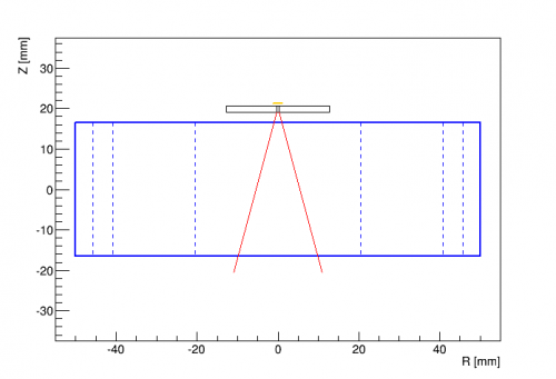 |  |  |
| Source and collimator arrangement | Red lines represent contours at 50% (z,r = 5.3,3.7 mm) and 90% (z,r = 21,11 mm) | Red lines represent contours at 50% (z,r = 0.4,1.4 mm) and 90% (z,r = 1.1,2.0 mm) |
Low energy spectrum
| |
| Here's an energy spectrum from 0-2 keVee from -196V data. Originally the only quality cut applied was a baseline cut, but that showed a large excess below 1keV that grew with decreasing energy. Looking at sample traces showed that most were on distinctly downward-sloped baselines. Many of these events were removed with an OF-integral agreement cut (in particular downward-sloped traces with relatively small pulses tend to have negative integrals). There still seems to be a bulge below 1keV which may still be poorly reconstructed events with downward-sloped baselines. |
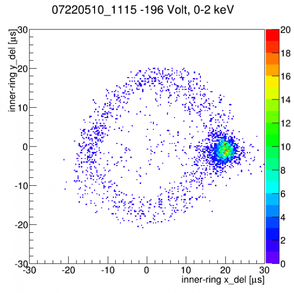 |
| Rather surprisingly much of the low-energy spectrum seems to be from the Am source rather than lab background as can be seen in this x-y delay plot. |
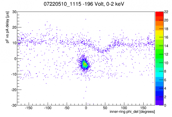 |
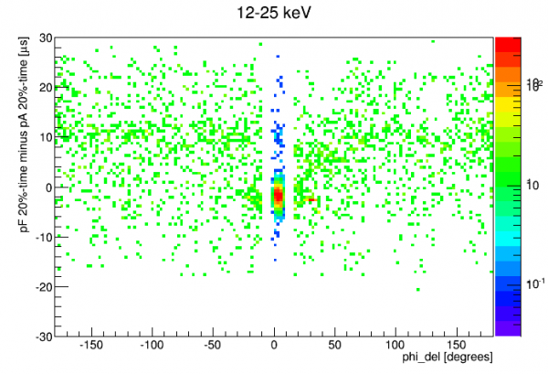
| Another way to see that much of the low energy spectrum is from Am-241 is this pF-pA delay versus phi delay plot. |
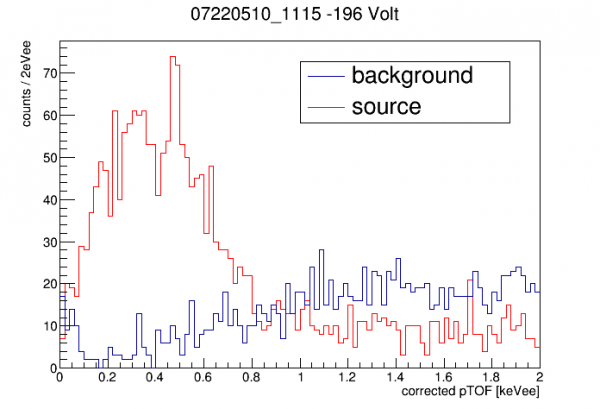 |
| Here we plot the Am-241 spectrum (selecting events based on position) and the background events (those failing the position selection). |
Geant4 simulations were run with a simulated Am source in its housing, one simulation of 60keV and another of 14keV. The 14keV shows very few events in the Compton spectrum at low energy, so I focus on the 60 keV spectrum which shows a significant low-energy Compton spectrum. To get simulated rates the data is normalized to 1 uCi activity and a branching fraction of 0.3592 is assumed (source: http://www.nucleide.org/DDEP_WG/Nuclides/Am-241_tables.pdf)
note: a previous version of this section was based on an error in the simulation - I thought I had set the macro for a silicon detector, but I left out an additional command necessary to implement the change, so it actually was germanium in the simulation. The Compton spectrum from 60keV in Ge is much, much weaker than in Si.
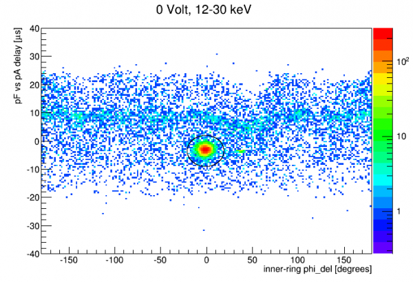 | 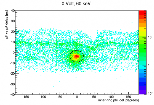 | 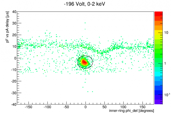 |
| An elliptical cut in pF-pA versus phi delay space selects the Am-source region. The same cut seems to work for the 60keV peak and lower-energy peaks in 0V data and also for the low-energy spectrum in HV data. Not surprisingly the 60keV peak is more smeared in position space so the cut doesn't work as well at that energy. | ||
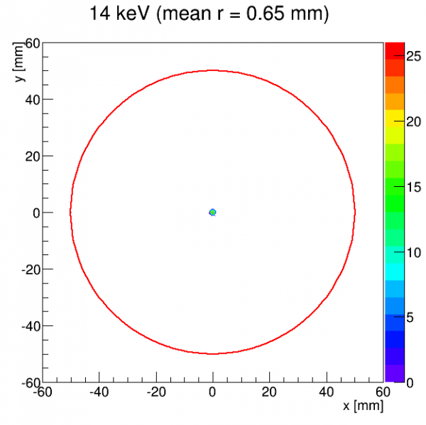 | 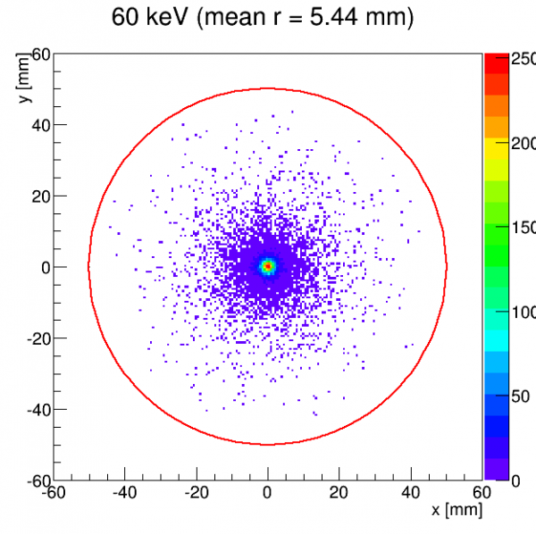 | 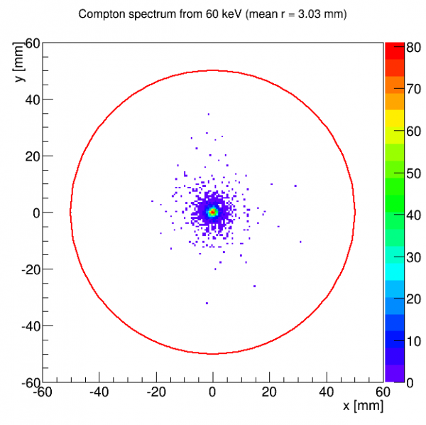 |
| Simulation gives a sense of how tightly resolved the Am-source position is expected to be for various energy ranges. | ||
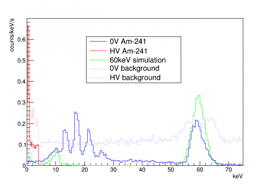
The plot above compares simulation to 0-V and HV data, with all histograms calculated in rate units (counts/keV/s).
Notes and comments:
- Data hasn't been corrected for write efficiency and cut efficiency. So the true rates in the data are probably higher than shown.
- For the 60keV simulation the 60keV peak has been widened to the observed resolution. The Compton spectrum at low energy has not been modified.
- The simulation shows a remarkably close fit to 0V data, considering the uncertainties in the simulation (for example the exact collimator hole size). The position selection is not as efficient for the 60keV peak so it's not surprising that that is lower in the data.
- Both the Am and background spectra in HV data below 4keV show anomalously high rates. This is stronger for the Am-source data. (In the 1-4keV range, Am-source rate is perhaps 4-5 times higher than expected, while background rate is perhaps 2.5 times higher.)
- In particular the bulge in the Am spectrum below 1keV is very high. Again I should investigate further whether this may be somewhat subtle data quality / reconstruction error issues.
Coincidence Test
Trigger signals from the NaI array are read out by DCRC4 along with phonon signals from S104.
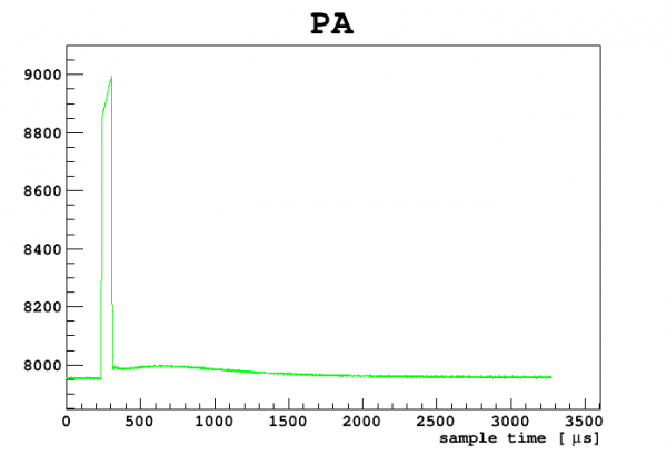 |
| example of trigger signal from NaI array as seen in DCRC4 |
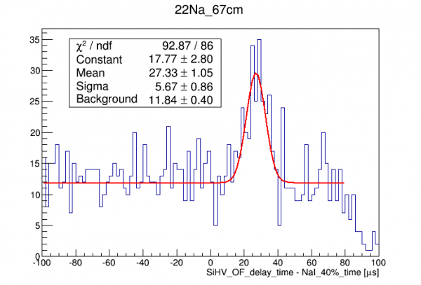
To test for coincidence and to study the time delays between phonon pulses and NaI array signals, we arranged the Na-22 source North of S104, level with the detector. The vertical part of the NaI array is South of the cryostat. The idea was to look for 1275keV gammas which scatter in S104 then leave S104 and hit the NaI array. We set up a trigger in the NaI array so that only three NaI detectors (#10, #11, #12) that are level with S104 are enabled to trigger, with an intended energy window of 950-1275 keV. Approximate amplitude/energy calibrations led us to an actual trigger window setting of 1300-2100.
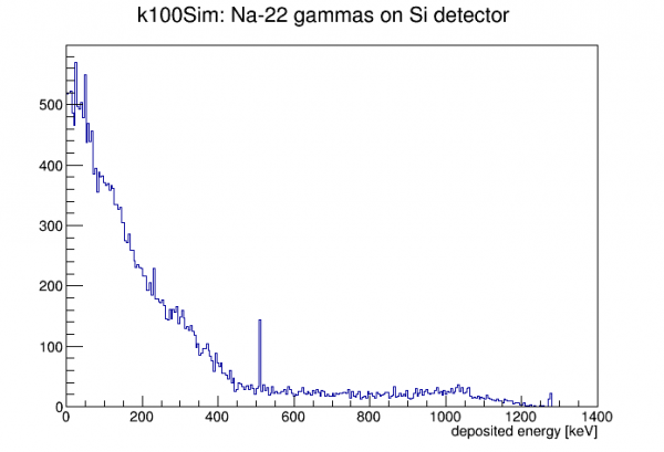 | 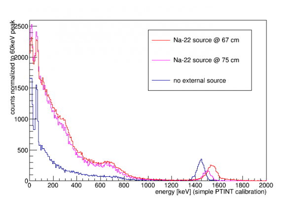 |
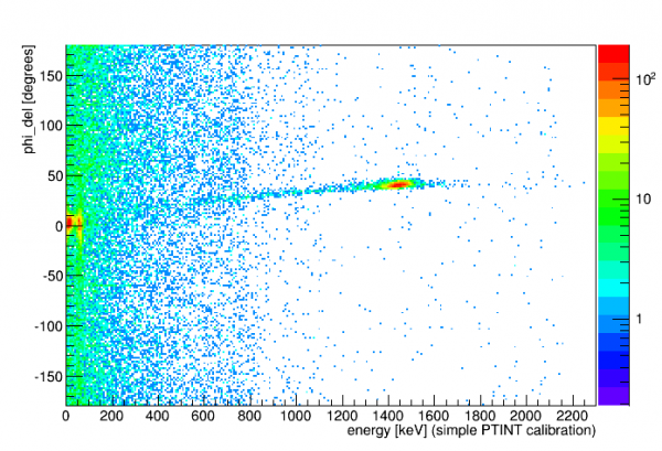
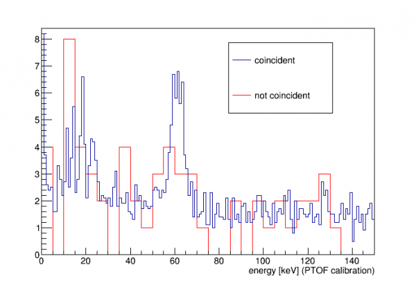
| Simulated spectrum of Na-22 on S104 and data from three series with and without the source. The energy calibration uses pT integral and the 60keV peak with no correction. Comparing simulation and data we can see that at high energies the calibration is a bit low. There is perhaps a hint of a 511keV peak in the red data spectrum showing up around 450 keV. The peak seen in data around 1500 keV (true energy may be closer to 3 MeV) is not related to the external source. More on this below. My guess is that this is alphas from Am-241, meaning we neglected to block the alphas from the source (either we forgot to put tape on it or the tape fell off). |
|
As it turns out the sim data suggests that this test is very inefficient. Of the events with hit in Si the fraction that also have hits >950keV in any of the three NaI detectors is only 0.12%. (The sim only considers single gammas from the Na-22 source - another possible coincidence is a 511 gamma hitting S104 and a simultaneous 1274 gamma hitting one of the NaI detectors. But this is even lower probability, 0.02%.)
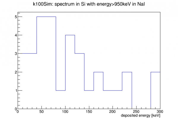 |
| This plot from the simulation shows the energy spectrum expected in S104 for events that pass the S104/NaI coincidence criterion. |
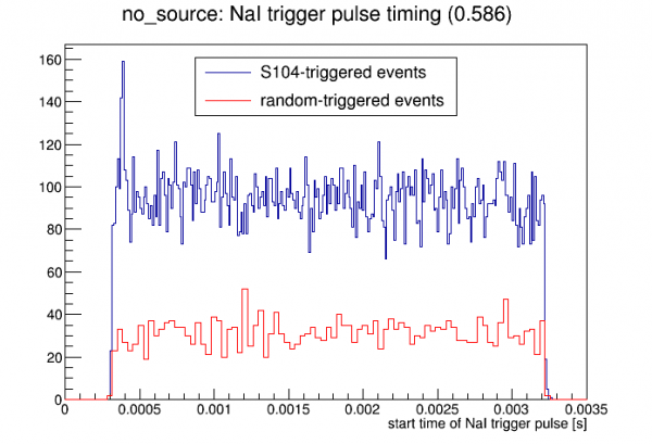 | 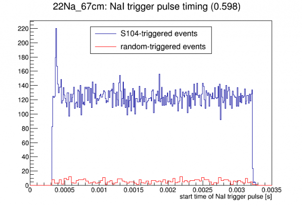 | 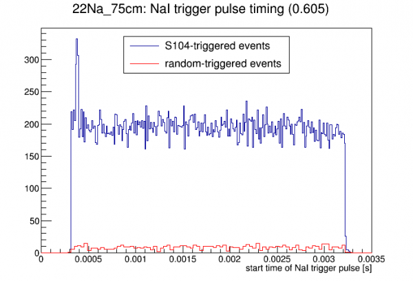 |
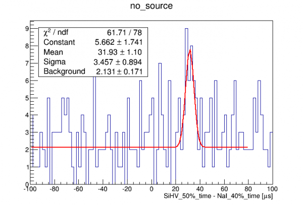
| After cuts removing NaI trigger traces that have pulses too early to calculate the baseline and selecting only traces with 1 NaI trigger, the plots above show the start time of the NaI trigger pulse for each of the three data series. In each case a peak is seen at the S104 trigger time, in S104-triggered events but not randoms, indicating the presence of coincident events. The number in parentheses is an estimate of how many events near the trigger time of 400 us are true coincidence rather than accidentals, based on how high the peak rises above the flat background. We see there's very little increase in this fraction with the source present - not too surprising after noting the poor efficiency of the coincidence setup. So, probably the coincident events we see are mostly from lab background (possibly muon showers and possibly lab background gammas scattering between S104 and the NaI detectors). |
||
 | 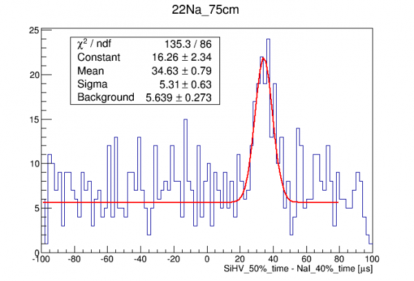 | 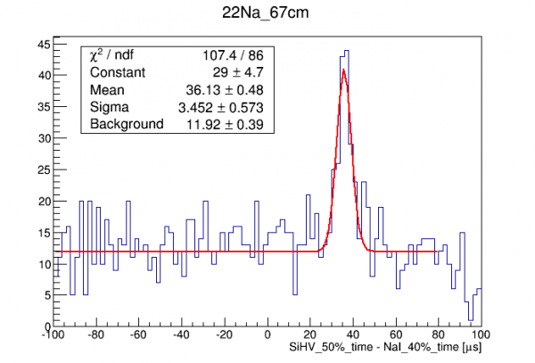 |
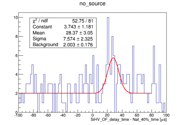 | 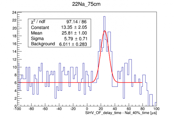 |  |
Muon coincidence
On June 17 we set up a muon coincidence test, configuring the three bottom NaI detectors (#21,22,23) to trigger at their saturation level, thus triggering mostly on through-going muons. S104 data was taken both using the standard phonon trigger and alternatively using the NaI trigger.
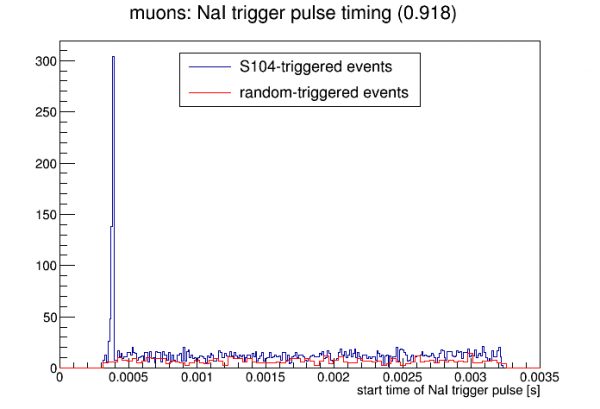 |
| In contrast with the Na-22 coincidence test, accidentals are quite rare. The coincidence peak rises far above the accidental continuum. |
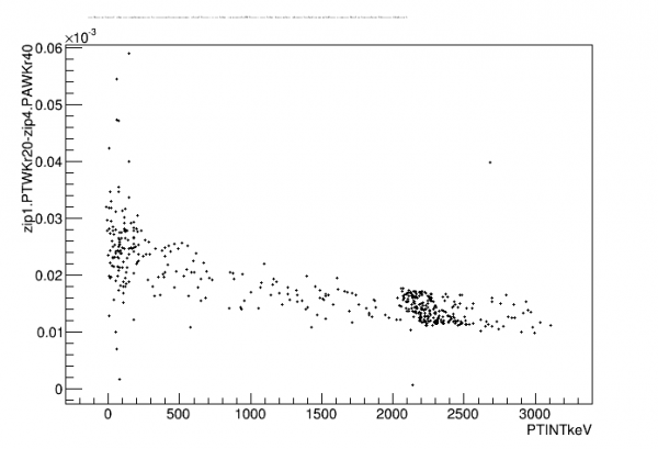 |
| With the Na-22 coincidence I saw no energy dependence in the NaI/S104 timing. But here it's clear that as we extend to muon energies there's a distinct energy dependence. I tried a few different combinations of walk algorithm parameters to see if there was a timing quantity independent of energy, but I didn't find one. (It's probably not very important to study the timing characteristics of highly-saturated events.) |
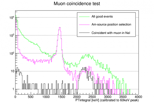 |
| For the most part the coincident spectrum is exactly as expected - a muon spectrum with a smaller high-energy tail because high-angle muons aren't tagged. But muon spectrum calculations give a low flat spectrum below the full-height peak extending all the way down to 0keV. Here there is a another population of coincident events at low energy, below around 200keV. It does not appear to be accidental. This suggests that some muons that hit the bottom detectors are accompanied by lower-energy secondaries that hit S104. |
Update: muon simulation
Shubham performed a Geant4 muon simulation on our k100Sim model. He threw muons from a 2m radius disk 3.5m above the center of the fridge world with a cos(theta) angular distribution (probably should have been cos^2) with energies ranging from 0.5 to 10 GeV.
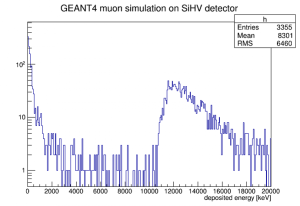 | 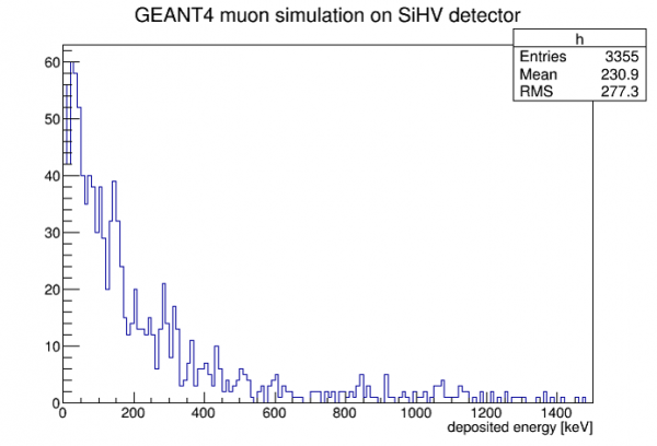 |
The spectrum in the SiHV detector is similar to my calculated spectra (which only consider muons hitting the detector and a fixed value for dE/dx) except there is an excess of events at low energy. The simulation results show that almost all of these events have no muon hitting the detector. Shubham concludes that mostly what we are seeing is bremsstrahlung radiation produced by muon interactions on fridge material that then hits the detector.
 |  |
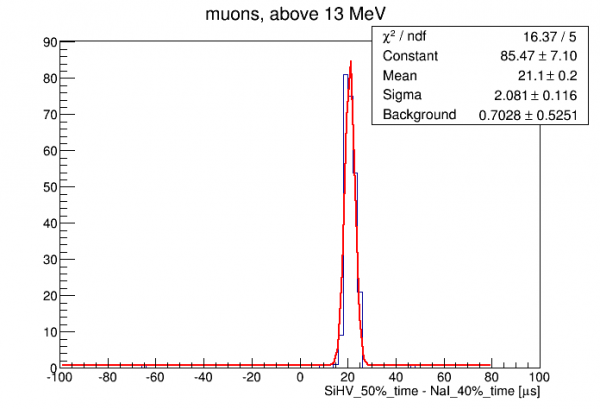 | 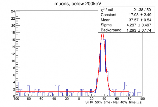 |
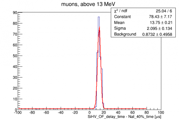
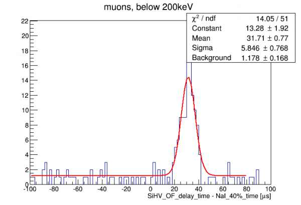
| Above the timing resolution is shown for the muon coincidence data, separately for the high energy events (full-height muons in S104) versus the low-energy events. (Top row uses the walk algorithm for the phonon timing, bottom uses the OF delay.) The high energy events show better timing resolution, but these highly-saturated events aren't really relevant to the n,gamma measurement. | |
Initial PuBe tests
On June 7 we finished the lead/poly shield and built the lead wall to shield the detectors from PuBe gammas. The setup was modified a bit from previous runs to accommodate the NaI array setup. To shield the bottom NaI detectors better we can raise the paraffin drum for the PuBe source about 12 cm with a wood platform (or stack 5 layers of poly, 12.7 cm high).
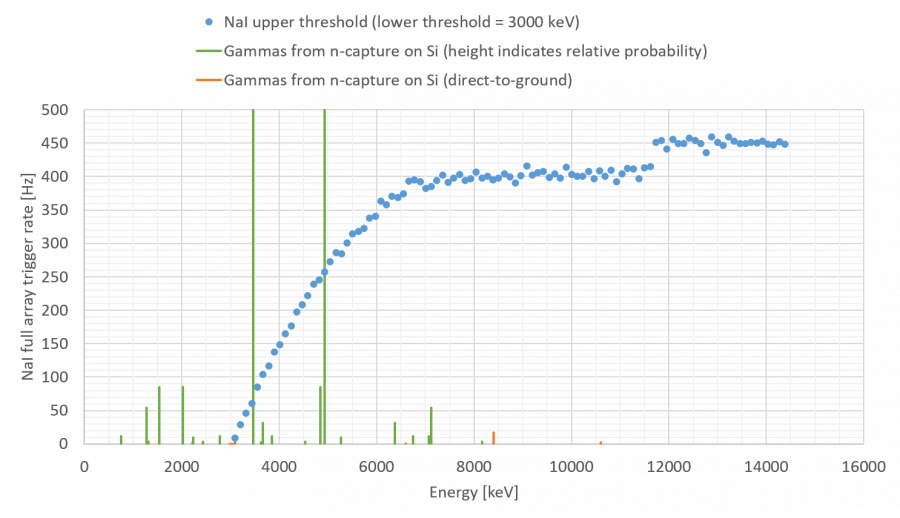
Two kinds of NaI rate test were performed: 1) fixed trigger window (nominally 3 MeV to just below saturation, which cuts out through-going muons) done separately for separate sets of 4 NaI detectors and 2) variable upper threshold with all NaI detectors triggering. Analysis in link below:
Basic observations:
- Raising PuBe does indeed reduce the rate of the bottom NaI row. But the improvement is not dramatic, which may indicate that much of the rate seen in NaI from PuBe is not direct gammas
- With PuBe elevated the total NaI rate rises steadily with upper threshold plateauing around 680 Hz at and above around 6.9 MeV
We also took some 0V data with S104, with and without PuBe present, finding the following trigger rates: 31 Hz without PuBe present, 61 Hz with PuBe present. These are calculated using the fraction of randoms that have pulses above a low-ish threshold.
Boron shielding tests
Boron shielding is expected to reduce the trigger rate in the NaI detectors. Many neutrons are expected to capture in the NaI detectors, producing high-energy gammas within the energy window for this experiment. Boron has a high neutron-capture cross-section and produces gammas of low energy, well below the energy window.
Description of how the boron shielding is made
On June 14 we placed fabric socks filled with Borax on and around the bottom row of NaI detectors (#21,22,23).
| Boron shield dimensions for bottom NaI row | ||||
|---|---|---|---|---|
| Diameter | Length | Weight | Number | Location |
| 2 in | 20 in | 0.79 kg | 6 | Crosswise on top surface of detectors |
| 2 in | 27 in | 1.20 kg | 2 | Along the sides of the detectors and wrapped a bit around the front (North side) |
We took NaI rate data with the same setup that was used before the boron was added. This reduced the trigger rate in the bottom detectors (with the wide 3 MeV to saturation trigger window used before) by about 40%.
As of June 15 six fabric socks were draped over the vertical stack of detectors (#1-20).
| Boron shield dimensions for vertical NaI stack | ||||
|---|---|---|---|---|
| Diameter | Length | Weight | Number | Location |
| 2 in | 100 in, segmented | 4.35-4.83 kg (only two were weighed) | 6 | Draped over the stack, hanging down on both sides |
As with the bottom detectors, for most detectors this reduced the rate by about 40%.
The bottom-most set of 4 detectors, #17-20, did not show as much improvement. We removed the South wall lead shield to inspect the socks. It turns out that one sock had folded back on itself at the bottom. We straightened them out and also tied a string around the bottom so that the socks would be tight against the detectors. (On the cryostat side they bowed out a bit before we added the string.) After this we took more scans. The rate for Detectors #17-20 fell by another 10%. Info here:
To help interpret the rate plots linked above here is a conversion from ADC value to keV:
Estimating accidental rate
Define the following:
- S = rate of clean (n,gamma) events in S104, signal events
- f = efficiency of tagging signal events with NaI array
- b = ratio of background rate in S104 region of interest to (n,gamma) rate
- T = total rate of triggers from NaI array
- r = coincidence timing resolution
(Note: if a signal event is accidentally tagged, we'll consider that a “good” event here. If energy information of the tagged gamma is available this would be a bad assumption.)
Then the fraction of tagged events in the S104 ROI that are accidental rather then signal is
accidental fraction = rTb/(rTb+f)
or if the accidental fraction is small, then
accidental fraction = rTb/f
Let's guess some numbers:
- r = 10 us. This is conservative.
- T = 400 Hz. This is the most recent rate measured from the NaI array with PuBe present and boron shielding present.
- b = 2. This is not known. This is a rough estimate based on Run 68 experience. Note that if the boron reduces the capture rate in S104 then b will be higher than in Run 68.
- f = 1/3. An estimate - Shubham's sims can improve on this.
Then accidental fraction = 0.024
The shape of the accidental spectrum may be roughly flat, in which case it would raise the signal spectrum in a uniform way. Or it could be quasi-exponential.
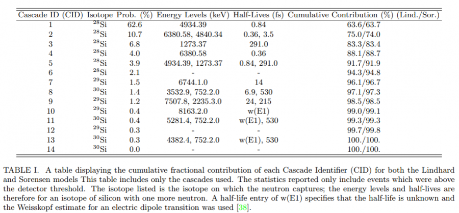
NaI trigger rate and gamma spectrum from Si neutron capture
Calibration: scaling series at different HV biases
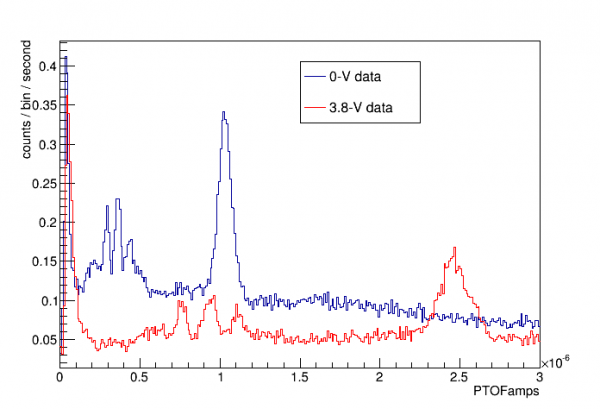
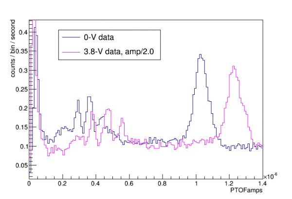
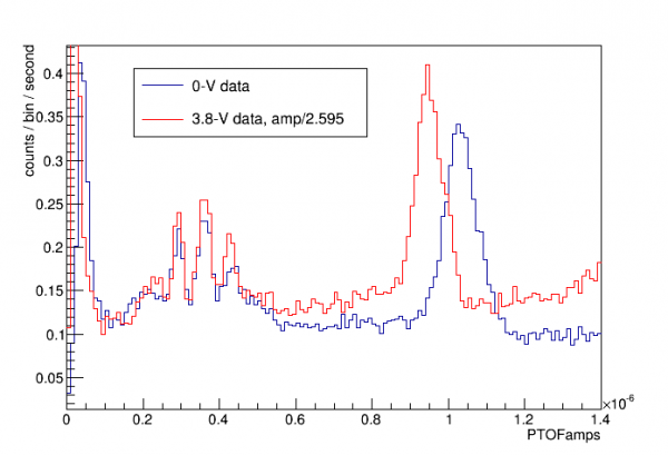
We'll try a calibration “ladder”, matching the 0V spectrum to a spectrum at higher bias, then matching that to a still higher bias, etc. The window for matching is between the noise wall and the point where saturation seems to become important.
Good set of NTL gains: 1, 2.7, 7.3, 20, 53 - this should be 0V, 6.4V, 24V, 71V, 197V
Ladder calibration
Data series at 0V, -4V, -24V, -65V, and -84V (the highest we can do under current conditions) were taken for the purpose of doing the ladder calibration.
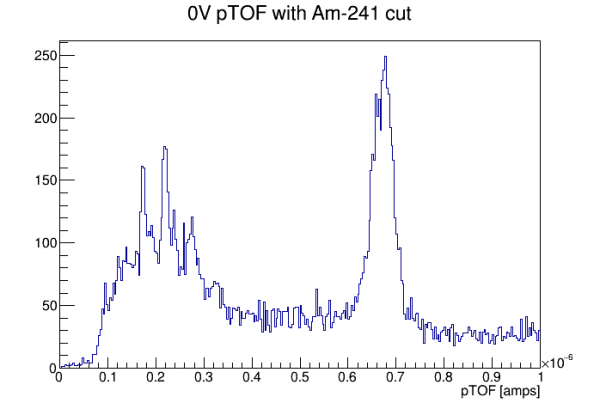 |
| First, 0V data with an Am-selection cut is used to calibrate energy. This calibration will be both keVee and keVpt |
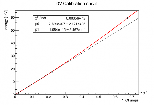 |
| The 14keV, 18keV, and 60 keV lines are used for a calibration curve, quadratic and fixed at (0,0). The black line shows the deviation from linearity. |
The hope is that the same keVpt can be applied to data at any bias, and an empirical NTL-gain factor can be determined by matching spectra. The keVpt calibration should only be considered valid up to 60 keV or a little above - that will apply at any bias, so that the valid region in keVee will be smaller each time we increase the bias. The threshold in keVee also gets smaller, so each new bias opens up a new lower portion of the spectrum.
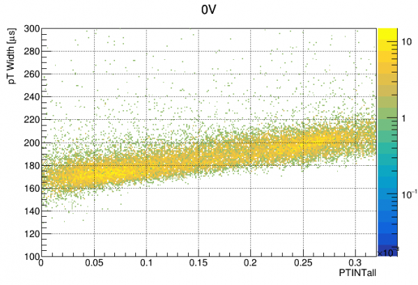
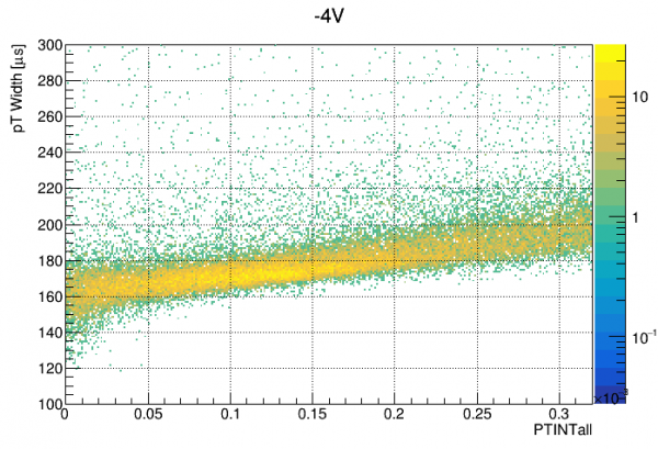
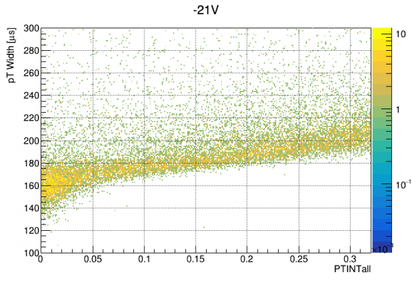
For the keVpt calibration to be valid from series to series, the pulse shape in the valid range shouldn't change much. This is investigated below by plotting pT pulse width versus integral at each bias:
 |  |  | 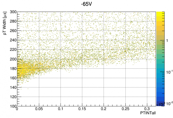 | 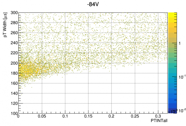 |
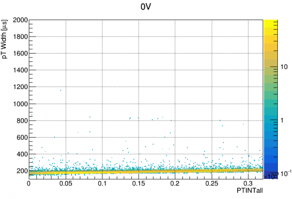 | 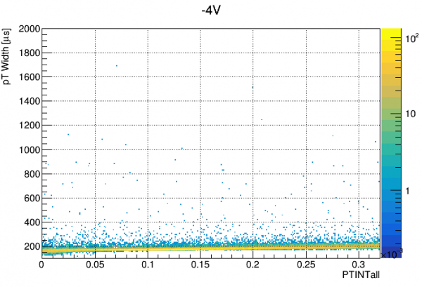 | 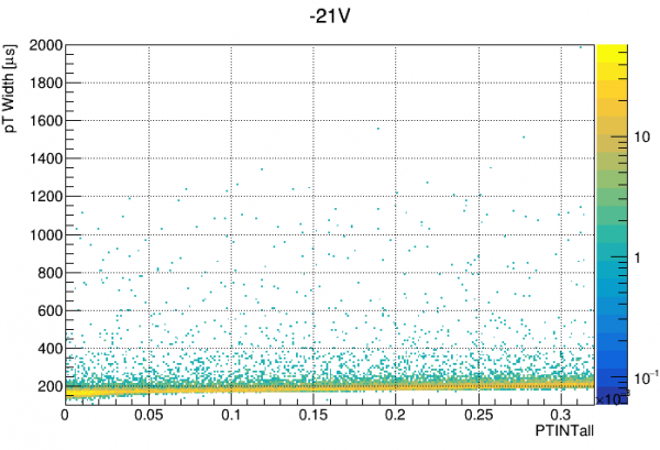 | 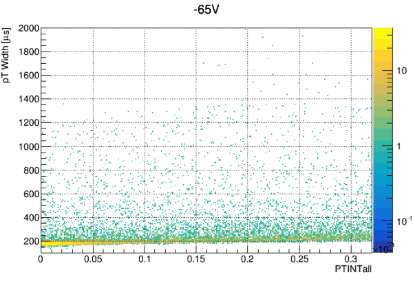 | 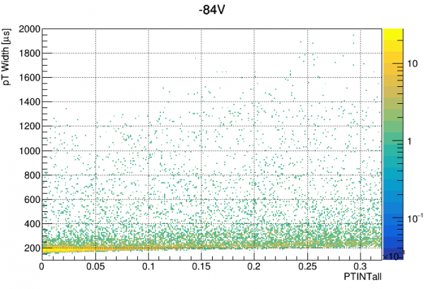 |
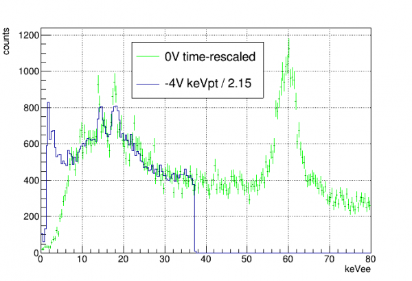 |
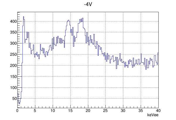 |
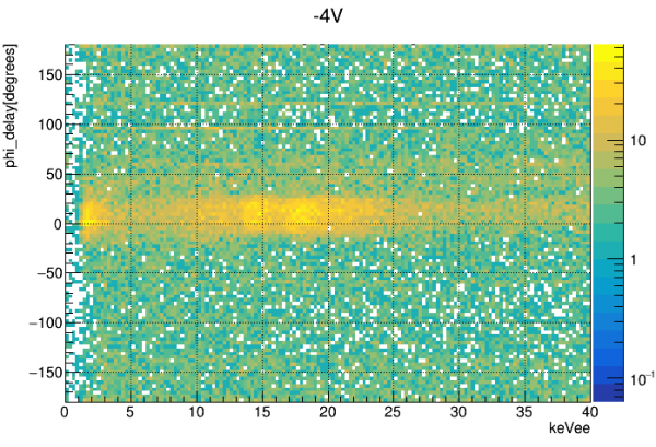 |
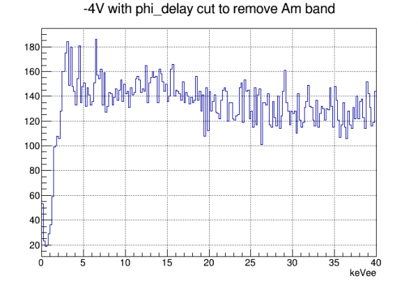 |
Calibration with baseline correction
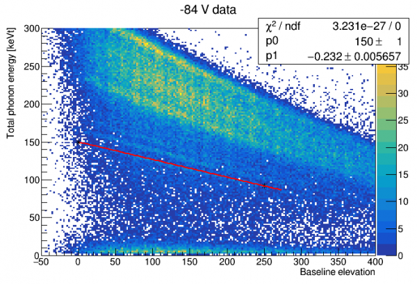
In HV PuBe data, we find that most events occur on significantly elevated baselines, because the event rate and the amplitudes are high, so usually the tail of the previous event has not entirely ended. As it turns out, if you plot amplitude versus baseline elevation you can clearly see Am lines!
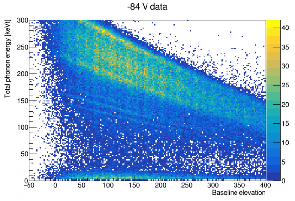
It is clear from the above that there is a problem with the ladder calibration, since there was no correction for baseline, and since the attenuation of amplitude gets larger each time you increase the bias. High energy events are shifted into the low energy region, so comparing rates is invalid (unless you can correct for baseline).
The attenuation with baseline elevation is clearly quite linear. We can make a fit, and then make a baseline-corrected energy:
 |  |
Since the 14keV and 18keV lines are now clearly visible, we can try to use them for a calibration as was done in Run 68. In that run we made an exact quadratic fit between those two lines and (0,0), as a simple curve that would be a linear energy-to-amplitude fit with an approximate correction for saturation effects. With the current detector, S104, saturation is stronger and the quadratic fit doesn't work - it gives a negative energy-to-amplitude curve at low energies. So instead I tried a different 2-parameter function, with a pole to model complete saturation at some energy above the visible Am lines. At low energies it reduces to a linear function, like the one used in Run68.
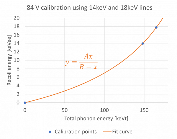
This calibration suggests a stronger NTL gain than the anomalously low values we got for the (incorrect) ladder calibration:
| implied NTL gain | 21.9 |
|---|---|
| empirical bias | 79.5 V |
This is much closer to the calculated detector bias - just 5% lower! (And considering that the estimated correction for leakage is 10%, this error is not very surprising.)
With this calibration we can recalculate the baseline resolution:
| energy resolution at 0 energy | 11.2 eVee |
|---|
Problems with data, probably caused by helium films
| NOTE: the report below is from an early period when we were first diagnosing the helium films problem. Later we found that we could fix this problem by suspending circulation, warming the fridge above 5K, pumping out the IVC, then recooling. This restored the phonon channels to good behavior for a period of about two days, after which we needed to do another pumpout. |
On 25 July the fridge failed due to an impedance blockage. The blockage was gone at 100 K so we cooled back down. We reached base but saw temperature instabilities (semi-periodic spikes) which suggested helium in the IVC. Also (though it wasn't noted at the time) the IVC pressure began to rise during the initial LHe transfer as the temperature fell below 20 K - this was happening in Run 74 and eventually led to a complete disassembly and replacement of the stripline elbow seal.
But - we found that the phonon channels still looked good, although they required significantly higher QET biases to get them into transition. We began taking data at different biases on 12 August.
Looking at the processed data shows that it is of much poorer quality. Amplitudes are suppressed by a factor of several, and energy and timing resolution is much worse. Also pulses are significantly more narrow.
The detector behavior seems to be consistent with a superfluid helium film on the detector:
- Reduced amplitude, poor resolution, shorter fall times all could be caused by a helium film on the detector surface
- The higher QET biases required at first hinted at a colder detector temperature (though the MC was not significantly colder). But maybe this is instead caused by the helium film increasing the thermal conductance between TES and detector.
- IbIs behavior seems overly sensitive to small changes in temperature. This could have to do with changes in the thickness of the helium film or something. Note that this sensitivity plagued us during Run 73 - when there was probably also a problem with helium in the IVC.
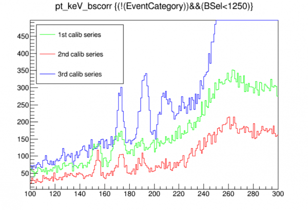
Calibration variation patterns
| Sep 16-17 Data Period | Aug 30-31 Data Period |
|---|---|
 |  |
 | 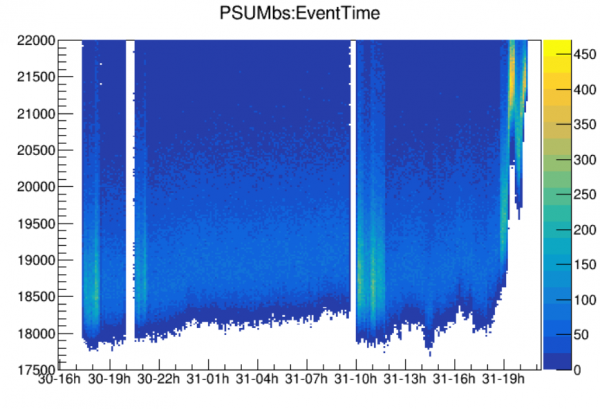 |
In both these data periods there is one calibration series showing much higher gain than the other two.
In both cases this outlier series occurs at a period where the phonon baselines dip.
| Sep 16-17 Data Period | Aug 30-31 Data Period | |
|---|---|---|
| Time that circulation started | 3:35 PM | 3:50 PM |
| Time next day that baseline dipped | ~ 10 AM | ~ 10 AM |
Notes:
- In the first period analyzed the outlier series was at an overall low baseline, but this is not the case in the second period
- In the first period there is evidence that the unusually high gain disappeared later in the data period
Oct 19-21 data period
During analysis I discovered that three channels (pB, pD, pE) had railed in the middle of the data period. Here I'll attempt an analysis using the three good channels to track changes in baseline and gain.
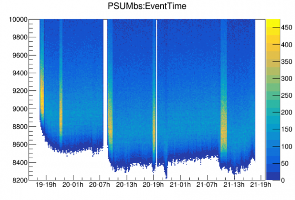 |
| note: baseline here is sum of pA+pC+pF only |
We see the initial dip on the day after the period starts. The table below shows that it occurs at approximately the same time after beginning circulation as the other two periods studied.
| Sep 16-17 Data Period | Aug 30-31 Data Period | Oct 19-21 Data Period | |
|---|---|---|---|
| Time that circulation started | 3:35 PM | 3:50 PM | 3:10 PM |
| Time next day that baseline dipped | ~ 10 AM | ~ 10 AM | ~ 9 AM |
There are five calibration series in the data period. The railed channels occur before the 4th calibration series (07221020_1846).
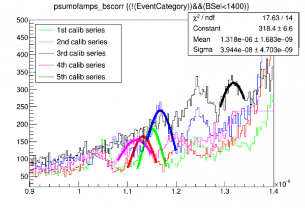
Oct 25-27 data period
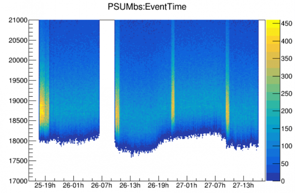
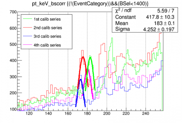
SiHV-triggered data
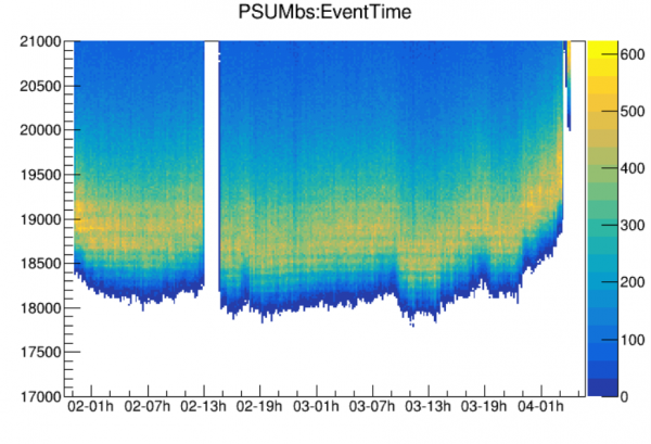
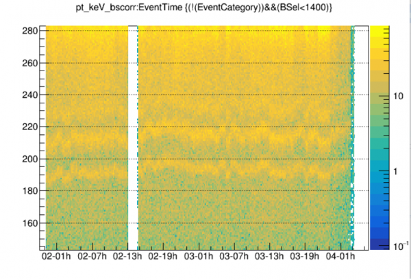
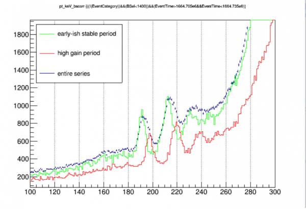
We have some long datasets triggered by the SiHV (Run68-style). These will allow us to see how the calibration varies in a continuous way, since the Am lines will be prominent throughout the series.
 |
 |
 |
Coincident spectra using only the early parts of the data periods, before the baseline dip
| Sep 16-17 data period |
|---|
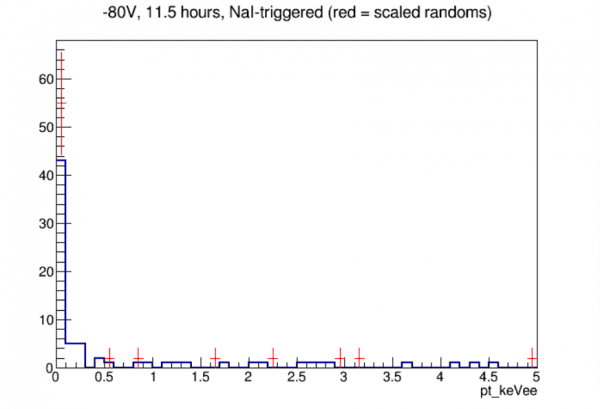 |
| total estimated efficiency: 0.190 |
| Four data periods |
|---|
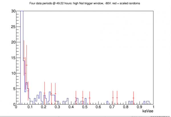 |
Coincident spectra, -80V with high NaI threshold, full data sets
Here I combine all -80V high-NaI-threshold data, full datasets rather then just early data:
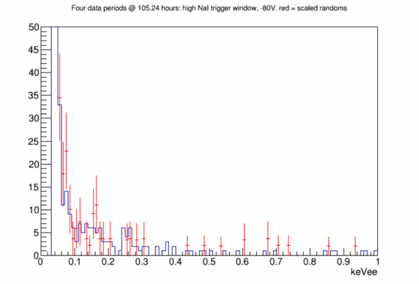
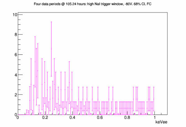
Extending the randoms background spectrum
In the analysis above I created the randoms spectrum to estimate the rate at which accidentals (as opposed to true n,gamma coincidences) sneak into our signal spectrum. I used the exact same cut criteria as for the triggered events, including a tight coincidence window (32 samples = 25.6 us). Here I try extending that, looking for random pulses in the full optimal-filter timing window, around 165 samples wide.
The plot below is an initial check of optimal filter pulse start time versus energy for one of the four datasets, with all of the relevant signal cuts applied:
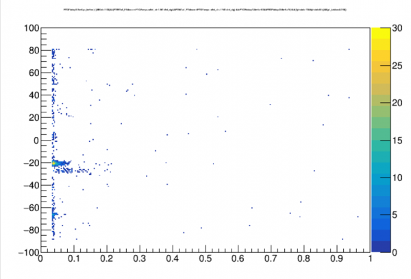
This combines both randoms and triggered events. The only cluster in time that we expect is near the coincident region for the triggered events. We see some of those in the 20-40 range on the vertical axis, at low energy. But there are more distinct clusters around -20 and -65. I haven't figured out why those are there. Likely it has to do with some form of noise at the beginning or end of a trace and some strange way that the optimal filter finds a preferred “start time”.
Comparing actual randoms spectra for different OF start time regions led me to create a cut to remove the biggest cluster near -20. With this cut I made a new signal-plus-randoms plot. Normalizing the randoms in this case is less straightforward, since it's clear there are “preferred” start times rather than random pulses being uniformly distributed in time. In the plot below I normalized the randoms with respect to how many more appear in this extended sample versus the original restricted sample. Alternatively I could have normalized based on how much larger the sampled time window is compared to the coincident window. In the latter case the randoms rate would be about 25% higher than what is seen below.
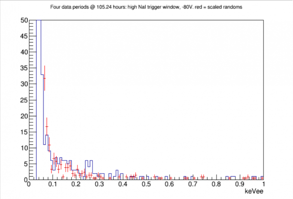
Comment: the two peak-like figures in the triggered spectrum that may be an indication of signal are not really visible in the randoms, which adds a little more confidence that the peaks really are signal.
NOTE: there's a high priority to look at traces for both random and triggered events in the region of interest, because there are probably clearly bad traces sneaking through that we don't yet have cuts for.
UPDATE: a look at some traces in the ROI revealed a number of bad events, usually with a first-samples glitch or a pileup event at the very end. Many of these were eliminated with a chisquare cut. See below for updated spectra. Bonus: the chisquare cut removes the strange clusters seen in OF start time.
Followup: we can add more stats by looking at triggered pulses that appear outside of the coincident window. These are essentially random pulses too.
Closer look at random hits in 80V NaI-triggered data
We’ve seen that the randoms spectrum in the ROI (which uses all the same cuts as the signal spectrum but selects randoms rather than triggered) has a similar shape to the signal spectrum with a somewhat lower rate. Anthony suggested that this might actually be signal events that we are just catching in the randoms. If they are mostly signal events, we might expect about 1/3 of them to have coincident NaI triggers, judging from the solid angle of the NaI array. I looked closer at the data to see.
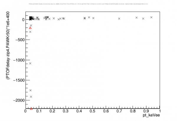
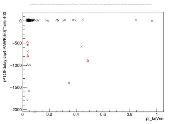
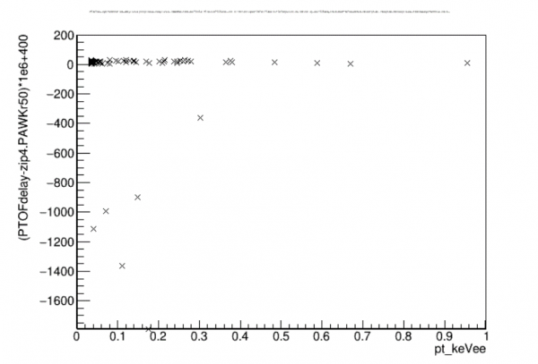
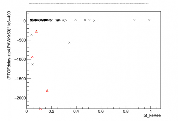
A simple cut to see if an NaI trigger is present is just to look at the max of the NaI trigger trace (zip4.PAWKmax). A few of the randoms below 1 keV do have NaI trigger pulses, but not many, as seen in the plots below (separate plots for the 4 datasets investigated). The cuts on the signal events require the SiHV pulse to be close in time to the trigger time. So we can also check whether the NaI trigger is close to the trigger time. As can be seen in the plots, none of the NaI triggers is close to the trigger time for the randoms that have NaI triggers. So it doesn’t look like any actual coincidences sneak into the randoms spectrum.
| Delay of NaI trigger pulse with respect to SiHV OF time for each of the four datasets | |
|---|---|
 |  |
| 0916-17 | 0830-31 |
 |  |
| 1019-21 | 1025-27 |
Note: it’s also seen that some triggered events have non-coincident NaI trigger times. But this is actually NaI pileup. The quantity I’m using to check the NaI time is from the walk algorithm (zip4.PAWKr50). When two NaI trigger pulses appear in the same trace there’s a pretty much 50-50 chance that the later one is slightly higher, so that the walk algorithm follows that pulse rather than the one that triggered the event. It’s easy to check using the integral of the trace (zip4.PAINTall) whether there are zero, one, or two NaI trigger pulses in the trace. For the triggered events that have apparently late NaI triggers, it’s always the case that there are 2 NaI trigger pulses. For the randoms it’s always just 1.
Coincident spectra with chisquare cut applied
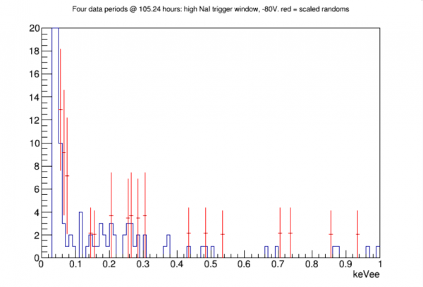
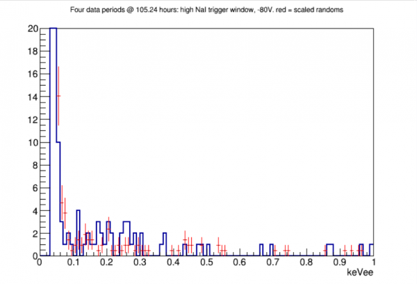
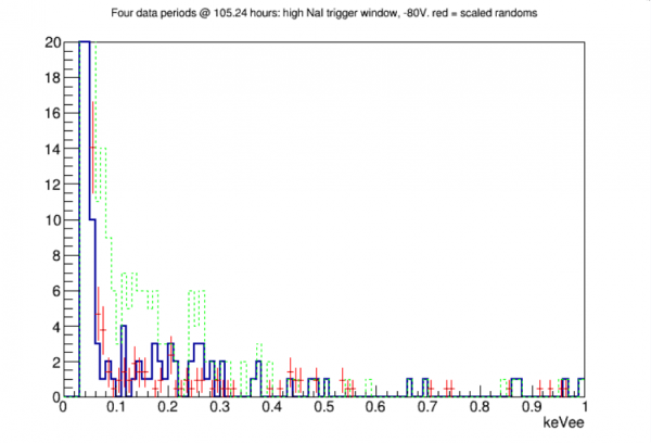
The chisquare cut cleans up the spectrum significantly. The usable analysis threshold is lower. But there is still a pretty big excess at low energy. We need to again look at raw traces for events passing the cuts.