Table of Contents
Read Rate versus Event Rate
Introduction
It's long been noticed that in standard self-triggered modes, the rate at which events are actually read and stored by the DAQ is significantly lower than the true event rate. This study attempts to quantify this and understand why it happens and whether it can be improved.
Standard running mode
Data from 2017 Dec 15 were taken in our current running mode: DCRCs 1,3,4 read out, with 3.2768 mS phonon traces and 51.2 μS charge traces, triggering on DCRC3pD (Side1pF), and with 150 μS set as a pileup rejection threshold in the MIDAS ODB.
Three 60-minute series were taken with 2000 initial randoms. An event rate was calculated from the initial randoms and a read rate was calculated from the triggered data. In each case an event was defined with the following selection: PEWKmax > 0.05e-6. This is a pulse-height threshold. By choosing a height quantity rather than an area quantity we avoid the problem that if the pulse occurs late in the pulse in a random event we may lose part of it and the area may fall under threshold. The height threshold is chosen to be low energy but high enough to be well above the trigger threshold.
Results:
| Event rate | 30.4 ± 0.9 Hz | ||
|---|---|---|---|
| Read rate | 23.26 ± 0.05 Hz | Efficiency | 76 ± 3 % |
| Read rate (retriggers removed) | 22.02 ± 0.05 Hz | Efficiency | 72 ± 3 % |
The “retrigger” cut will be described further in a later section.
Ruled-out mechanisms for loss of read efficiency
Pileup can reduce the efficiency for reading events. If events are sufficiently separated, the DAQ should trigger on each pulse separately even if two appear in a single trace. There are two levels at which pileup is rejected by the DAQ: at the DCRC firmware level (described further below) and at the MIDAS DAQ software level. For the latter our standard separation time limit is 150 μS (which is longer than the DCRC limit). At the 30.4 Hz event rate, there is only a 0.45% probability that an event is followed by another within 150 μS. Even if the DAQ throws out multiple events for every pileup, it should only be a few-% effect. Thus pileup cannot explain the low read efficiency (assuming that the pileup identification is accurate).
Trigger bursts occurred in this data set because the channel we triggered on has a strong oscillation regime high in its transition, so that when high-energy events like muons occur the TES gets driven into the oscillation regime and the DAQ triggers on the oscillations as the TES settles back down to its operating point. These extra triggers produce dead time because for each event the pileup rejection window is applied. However the total trigger rate for this data was only about 30 Hz, so the effect should be around 1%.
Random triggering mode
A non-standard running mode is to set random triggering, so that the MIDAS DAQ reads events at random times at a fixed user-chosen rate. On 2017 Dec 10 we experimented with high randoms rates to see whether the read rate kept up with the random rate. The setup (number of DCRCs, trace lengths) was the same as above. On 2017 Dec 15 we tried this again but with all the trace lengths reduced by half. We found that if the rate was set too high, the DAQ could not keep up – there was a saturation frequency:
| Standard trace lengths saturation frequency | 67 Hz |
|---|---|
| Half trace lengths saturation frequency | 110 Hz |
These seem to represent the limit at which the DAQ system can read out events. Naively one might expect the readable rate to increase by 2× when the trace lengths are decreased by half, but the improvement is only about 64%. So there is probably some per-event overhead.
So there is a limit to how fast the DAQ can read events, but it is well above our typical event rates.
Running with no pileup rejection
We took three series of data before the standard three series on Dec 15 with one difference: the separation time limit for pileup rejection in the MIDAS ODB was set to 0. This turns off the MIDAS pileup rejection. The event rate and read rate were calculated as before.
Results:
| Event rate | 30.4 ± 0.9 Hz | ||
|---|---|---|---|
| Read rate | 38.26 ± 0.06 Hz | Efficiency | 126 ± 3 % |
| Read rate (retriggers removed) | 28.99 ± 0.05 Hz | Efficiency | 95 ± 3 % |
The initial measurement of the read rate was higher than the event rate. This is due to “retriggering”: a pulse is read out at two slightly different times and recorded as separate events.
If we remove the retriggers from this data we find our remaining read efficiency to be much closer to 100%. Below I describe the retrigger selection.
Retrigger Cut
The principle behind the retrigger selection is to identify successive events in which the pulse size and shape is exactly the same. I used a combined quantity from the RQs that expresses the absolute maximum of a trace in ADC units:
PEWKmax*PEnorm+PEbs
The peak height is taken from the RTFT walk algorithm. This is a relative height, with the baseline subtracted. The above converts back to ADC units and adds the baseline back on.
Looping through all the data I built a new TTree which stores the absolute maximum of the event's PE trace and also the previous trace. If these values match within 0.1 ADC units, the event is tagged as a retrigger. (The resolution is better than 1 ADC unit because the walk algorithm effectively interpolates between samples.) The TTree also records the RTFT times of the maximum and the previous trace's maximum. For the 6 hours of data in this set the retrigger cut tree takes a few minutes to generate.
| Examples of retrigger tagging | |
|---|---|
| Data with 150 μs pileup rejection | Data with no MIDAS-level pileup rejection |
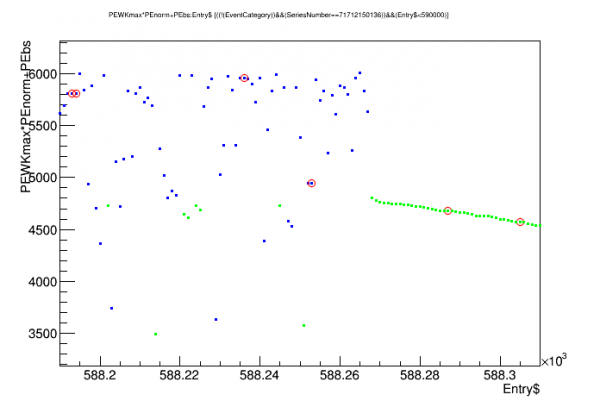 | 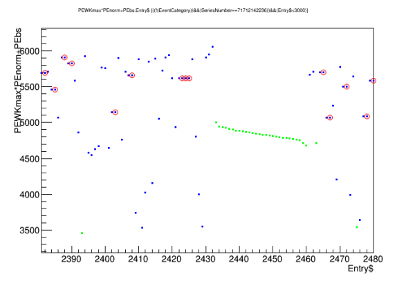 |
| Blue: events above selection threshold Red circles: tagged as retriggers Green: events below selection threshold |
|
The plots above show the absolute trace heights for two sets of successive events (left is data with the standard pileup rejection, right is with no MIDAS pileup rejection). Red circles show events tagged as retriggers. In some cases there are many retriggers for one pulse. (Also shown in green are low-energy events, below the PEWKmax>0.5e-6 selection threshold for measuring rates; the downward-sloping green segments are the trigger bursts mentioned previously.)
More retriggers are seen in the data with no pileup rejection (24.2%) than in the data with pileup rejection (5.3%).
Time Separation between Retriggers
The times within the trace of the trace maximum, as calculated by the RTFT algorithm, are stored in the retrigger cut tree for an event and the event immediately preceding it. The difference between the two should give the time between the retrigger and the previous trigger. These are plotted below:
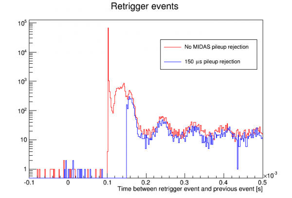
Notice that with the 150 μs pileup rejection applied, there is a sharp cutoff at 150 μs in the time separation. With no MIDAS pileup rejection, there is still a cutoff but at a lower point. There is a huge spike in pileups at a specific time separation, shown more clearly below:
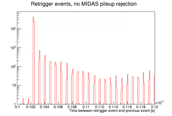
The large peak in separation time between trigger and retrigger is at 102.4 μs, which is exactly 128 samples. This arises from the DCRC firmware. The basic trigger condition is satisfied at a rising point in the trace, but the firmware also applies a trigger inhibit countdown, so that when the basic trigger condition is first satisfied there is a pause of 128 samples before another trigger can be issued. This will be described further below. It amounts to something very similar to a pileup rejection.
DCRC triggering algorithm
When the DCRC is set to trigger on a phonon channel there are three user settings applied (with the following typical settings): Baseline Length (16), Sample Length (5), Threshold (14). Usually we keep Baseline and Sample lengths at these settings and only adjust the threshold. The firmware essentially keeps calculates a running average of the amplitudes of the last [Sample Length] samples and of the [Baseline Length] samples before that. If the difference between the two averages exceeds the threshold the basic trigger condition is satisfied. However the basic condition will be satisfied for the entire time that the pulse is rising, and we don't want to trigger on every sample - so a trigger inhibit of 128 samples is applied. This number is not user-adjustable.
Using raw traces, I attempted to recreate the trigger logic by scanning through the trace of the triggered channel. Applying the above logic I found the basic trigger condition was first satisfied at very nearly Sample #500 (400 μs), which is the user-selected trigger time within the pulse. If I used the actual threshold it did not work as well - using a threshold twice as high as the user setting worked better, with the trigger position usually at 500, sometimes 499 or 501.
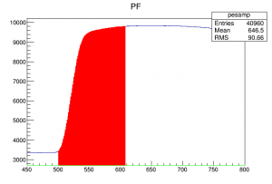
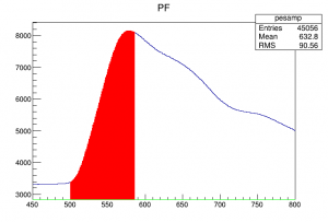
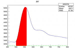
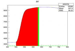
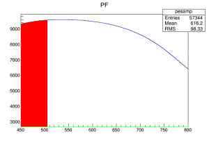
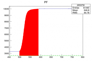
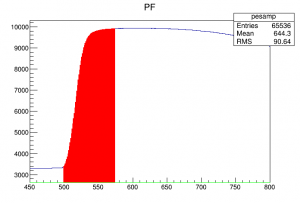
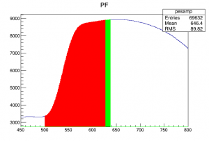
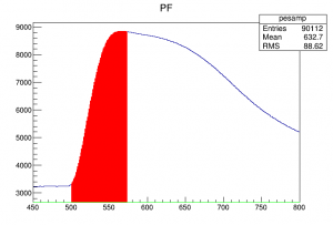
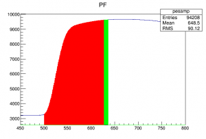
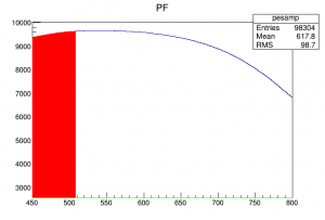
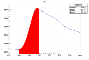
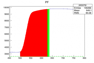
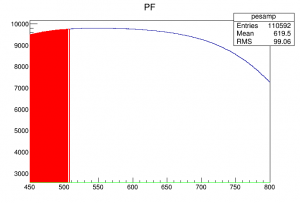
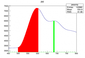
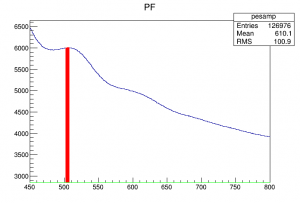
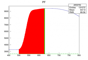
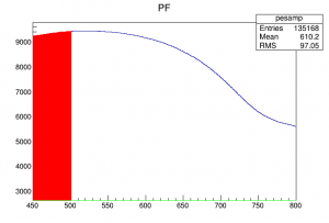
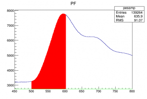
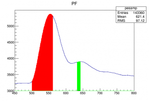
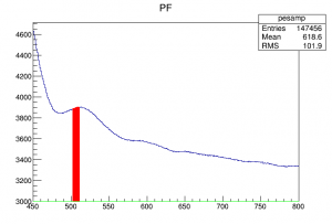
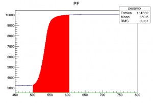
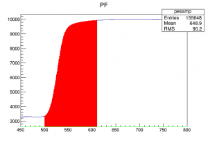
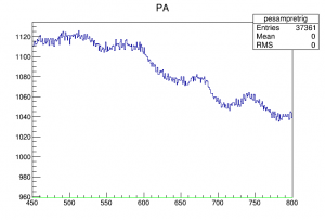
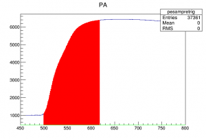
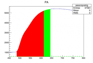
Shown below are plots of consecutive traces of the triggered channel, using the data with no MIDAS pileup rejection. The traces are zoomed in to the region around where the trigger should be. The area shaded red is the region in which the basic trigger condition is satisfied. Green indicates a region in which the trigger condition is satisfied and it is more than 128 samples past the first time it was satisfied.
| Traces from the triggered channel in data with no MIDAS pileup rejection | ||||
|---|---|---|---|---|
 |  |  |  |  |
| 50105 ↑ | 50106 ↑ | 50107 ↑ | 50108 ↑ | 50109 ↑ (tagged as retrigger) |
 |  |  | 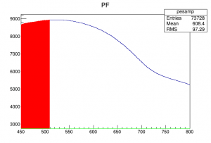 | 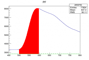 |
| 50110 ↑ | 50111 ↑ | 50112 ↑ | 50113 ↑ (tagged as retrigger) | 50114 ↑ |
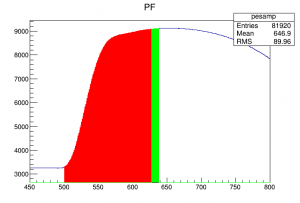 | 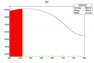 |  |  |  |
| 50115 ↑ | 50116 ↑ (tagged as retrigger) | 50117 ↑ | 50118 ↑ | 50119 ↑ (tagged as retrigger) |
 |  |  |  |  |
| 50120 ↑ | 50121 ↑ | 50122 ↑ (tagged as retrigger) | 50123 ↑ | 50124 ↑ |
 |  |  |  |  |
| 50125 ↑ | 50126 ↑ (tagged as retrigger) | 50127 ↑ | 50128 ↑ (tagged as retrigger) | 50129 ↑ |
 |  |  |  | |
| 50130 ↑ | 50131 ↑ (tagged as retrigger) | 50132 ↑ | 50133 ↑ | |
| X-axis in samples Red: satisfying the basic DCRC trigger condition Green: satisfying the basic DCRC trigger condition and 128 samples later than initial trigger |
||||
In several cases above the DCRC issued a retrigger. For example, in Event 50112, the basic DCRC trigger condition is satisfied for a little more than 128 samples, so the trigger resets and a second trigger, Event 50113, is triggered. (The trigger logic I applied to shade 50113 red applies for the entire early part of the pulse, but the DCRC did not issue the retrigger until the the point 128 samples after the previous trigger.)
So, in the case in which we turn off the MIDAS pileup rejection (and trigger on a single phonon channel), the mechanism by which we get retriggers is clear: the DCRC will issue a retrigger if the rising part of the pulse lasts longer than 128 samples. As can be seen above this is pretty frequent for this detector, or any detector with phonon risetimes longer than 102 μs.
In the cases 50125/50126 and 50130/50131 the retrigger is on an oscillation on the tail of the pulse. I would still call this a retrigger because it is clearly the same pulse. But it's a somewhat different case because the retrigger is on a second rising portion. In that sense it is similar to a true pileup (two different pulses close to one another in time, i.e. within one trace length).
Understood this way it is clear that the retriggering phenomenon will depend on channel and energy, since it depends on pulse shape. Different energy regions will likely retrigger at different rates.
Possible mechanism for losing events
When the MIDAS pileup rejection is on, with e.g. the usual time separation limit of 150 μs, it will affect both true pileup events and DCRC retriggers. If the MIDAS algorithm rejected only the retrigger, i.e. only the second of two closely-separated triggers, it would work something like my retrigger cut. But the algorithm currently in use, in the DAQ program triggerfe2.c, removes both of two closely-separated triggers:
if(real_time_difference_next < pileup_cut){
	if(real_time_difference_prev < pileup_cut){
		#ifdef PILEUP_COMMENTS
			printf("PILEUP--both the previous and next event are within %f seconds of this one\nWill not read these waveforms\n\n", pileup_cut);
		#endif
	}
	else{
		#ifdef PILEUP_COMMENTS
			printf("PILEUP--the next event is within %f seconds of this one\nWill not read these waveforms\n\n", pileup_cut);
		#endif
	}
	return TRUE;
}
if(real_time_difference_prev < pileup_cut){
	#ifdef PILEUP_COMMENTS
		printf("PILEUP--the previous event is within %f seconds of this one\nWill not read these waveforms\n\n", pileup_cut);
	#endif
	return TRUE;
}

return FALSE;
An event is tagged as pileup if it is close to the previous trigger or it is close to the next trigger.
Why was triggerfe2.c written to reject both events in a pileup? Likely to make analysis easier - it's difficult to reconstruct the energy of events in pileup, and it will likely be removed in analysis anyway. It's also the case that if the event rate (and separation time limit) are small enough there will only be a small effect on efficiency.
But the pileup algorithm responds to DCRC retriggers too. In these cases the first event is not typically distorted - it is a good event. Only the second event should be removed. And, importantly, the retriggers can occur at significantly higher rates than pileup. So if both the first event and the retriggered event are removed, there can be a strong drop in efficiency.
Examination of the first sections of this note supports the idea that this is why we get lost events when the MIDAS pileup rejection is on. The data with the MIDAS pileup rejection off shows that 26% of events are tagged as retriggers. It could be that only 21% are true DCRC retriggers, since when the cut is applied there is a 5% efficiency loss (the other 5% may be true pileup or accidental). The data with the standard MIDAS pileup rejection has a 24% efficiency loss.
This gives a likely explanation for the lost efficiency: the standard MIDAS pileup rejection algorithm removes DCRC retriggers, but also the original event that produced the retrigger. DCRC retriggers occur with significant frequency, so this is a significant hit to efficiency.
Solving the efficiency loss problem
Probably the most logical way to solve the problem is to modify the MIDAS pileup rejection algorithm so that events are removed as pileup only if their triggers are close to the previous trigger. Events close to the next trigger will be retained. This would modify how pileup is treated: if two pulses fall within the time limit, the trigger on the first of them will be retained - but the trigger on the second one will be removed. This would allow some “junk” events in that would otherwise be removed.
Another solution would be to not use the MIDAS pileup rejection, and apply a retrigger cut at the analysis stage. But if we choose not to use MIDAS pileup rejection, it wouldn't make any difference if we modified the algorithm - so we may as well modify it anyway. Then we would have the choice of whether to use it or not. It's unlikely that we would want to use it in its current form because of the efficiency loss.
A third solution would be to modify the DCRC firmware, perhaps to allow a user-settable length for the number of samples after a trigger during which the trigger is inhibited. This would be relatively difficult given our lack of expertise in writing firmware.
Channel- and energy-dependence of the efficiency loss
As stated previously, the retriggering rate will likely vary with channel and energy. If events were lost in a random way we would have some confidence that our energy spectra have the correct shape. But with the efficiency loss caused by the MIDAS pileup rejection algorithm and the DCRC retriggering, our spectra will likely not have the correct shape: the efficiency will be energy dependent.
Also we have seen in this run that in the standard running mode the spectrum seems to vary significantly with the channel on which we trigger. On 2017 Dec 11 we six data series each triggering on a different channel. There were significant differences in the spectra produced, even at high energies where the trigger threshold should be irrelevant:
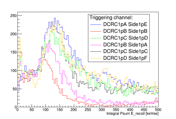 |
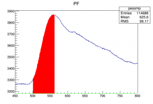
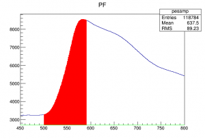
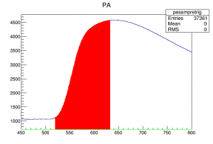
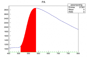
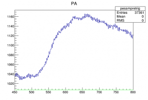
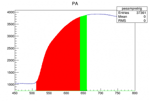
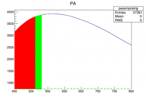
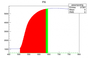
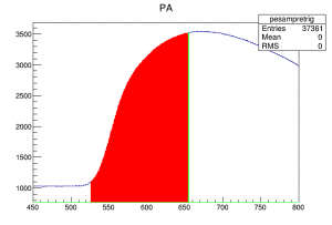
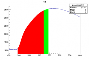
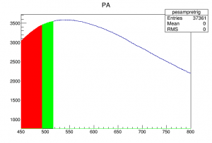
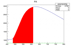
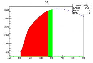
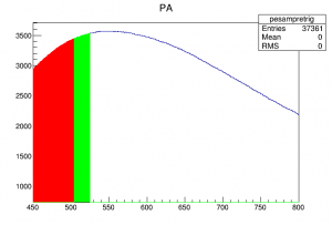
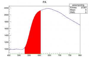
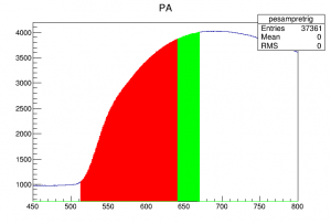
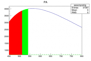
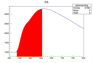
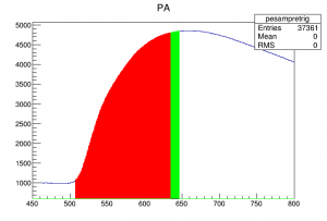
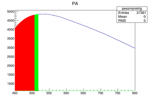
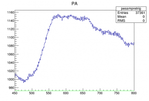
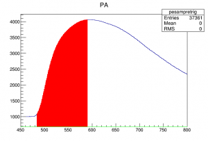
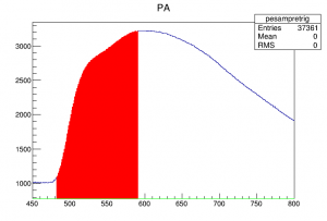
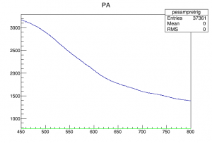
Triggering on DCRC1pB, for example, seemed to behave as though it had not only a minimum threshold but also something like a maximum threshold, since the high energy spectrum seemed suppressed. Below are plots of DCRC1pB traces for the PF-triggered data with not MIDAS pileup rejection, the same events shown in the previous section. The trigger logic is applied to DCRC1pB.
| Traces from DCRC1pB (Side1pA) in data with no MIDAS pileup rejection and DCRC3pD (Side1pF) trigger | ||||
|---|---|---|---|---|
 |  |  |  |  |
| 50105 ↑ | 50106 ↑ | 50107 ↑ | 50108 ↑ | 50109 ↑ (tagged as retrigger) |
 |  |  |  |  |
| 50110 ↑ | 50111 ↑ | 50112 ↑ | 50113 ↑ (tagged as retrigger) | 50114 ↑ |
 |  |  |  |  |
| 50115 ↑ | 50116 ↑ (tagged as retrigger) | 50117 ↑ | 50118 ↑ | 50119 ↑ (tagged as retrigger) |
 |  |  |  |  |
| 50120 ↑ | 50121 ↑ | 50122 ↑ (tagged as retrigger) | 50123 ↑ | 50124 ↑ |
 |  |  |  |  |
| 50125 ↑ | 50126 ↑ (tagged as retrigger) | 50127 ↑ | 50128 ↑ (tagged as retrigger) | 50129 ↑ |
 |  |  |  | |
| 50130 ↑ | 50131 ↑ (tagged as retrigger) | 50132 ↑ | 50133 ↑ | |
| X-axis in samples Red: satisfying the basic DCRC trigger condition Green: satisfying the basic DCRC trigger condition and 128 samples later than initial trigger |
||||
DCRC1pB (Side1pA, the outer ring) apparently has slower risetimes than DCRC3pD. Retriggers are more common. Moreover, examining the DCRC1pB retriggers, they occur when the center channel, DCRC3pD (Side1pF), has higher amplitudes. This probably explains why the DCRC1pB-triggered spectrum is suppressed at high energies - for high energy events, DCRC1pB usually retriggers.
Improved efficiency with modified trigger algorithm
A modified version of the MIDAS trigger front-end was written with a pileup rejection algorithm that only rejects an event if it triggers close in time to the previous event. If it triggers close to the next event, it is retained.
On 2017 Dec 21 we took data with the standard 150 μs pileup rejection limit, three 60-minute series with the old algorithm, three 60-minute series with the new one. The event rate and read rate was calculated as before.
Results:
| Event rate | 30.3 ± 0.9 Hz | ||
|---|---|---|---|
| Read rate, old algorithm | 21.87 ± 0.05 Hz | Efficiency | 72 ± 2 % |
| Read rate, new algorithm | 28.18 ± 0.05 Hz | Efficiency | 93 ± 3 % |
The new algorithm comes much closer to retaining the full event rate. The read rate is still a bit less than the event rate – I don't yet know why. At a 30 Hz rate the pileup rejection should reduce the efficiency by 0.45%, not enough to account for the loss.
The retrigger cut was applied to this data. A quick check of events tagged as retriggers showed that most are true pileup, and as such should not be removed to calculate the rate. Some retriggers are due to the oscillations in PF after a muon, and these probably should be removed (assuming that the oscillations fall below the amplitude threshold applied to count events with a pulse, which they likely do). So the read rate is probably somewhat overestimated.
Triggering on multiple channels from multiple DCRCs
In all of the above measurements we triggered on only one phonon channel. An OR trigger on multiple channels may be desirable in some cases. Triggering on multiple channels on the same DCRC should work the same as triggering on only one - the DCRC will issue triggers for either channel, and the inhibit from one channel may or may not affect the other, but the MIDAS trigger front-end should reject pileup in the usual way.
However the trigger front-end works one DCRC at a time. So the pileup rejection won't be able to catch multiple triggers on the same event coming from different DCRCs.
We took test data triggering on two DCRCs. The read efficiency was 117%, indicating retriggering. (With only one channel triggering the read efficiency is 93%.)
As described above I applied a retrigger cut, which looks for identical sized pulses in consecutive events. This did not work to remove the retriggers in this case because as we had seen in Run 65, the DAQ will write all events triggered from one DCRC in a bunch, then move on to the next DCRC. Hence identical events from the two DCRCs are separated by a bunch of events. A modified retrigger algorithm found that identical events tended to be separated by 65 events on average, with a rather wide scatter. Some low-energy events only triggered on one DCRC or the other.
One would expect that events above threshold would trigger on each DCRC, so that the read efficiency should be about double when triggering on two DCRCs. But it was only elevated by about 23%. An explanation comes from the overall rate. The trigger thresholds were set rather low, so that there were a lot of noise triggers. The read rate in the 1-DCRC case was 44 Hz. Doubling this to 88 Hz would exceed the limit we found using randoms in the current setup: around 65 Hz. And indeed in the 2-DCRC case the read rate was 69 Hz, so it appears it was saturated.
| Retriggering example in data triggering on two DCRCs |
|---|
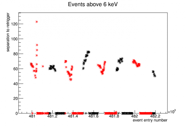 |
The figure above is a scan of 500 events above threshold looking for retriggers. The vertical axis shows the number of events separating an event from its retrigger, if found - events at 0 on the vertical axis are ones where a retrigger was not found. The color coding indicates time chunks. Plotting the EventTime shows that data is clustered in chunks separated not by 1 second (the resolution of EventTime) but rather by 2 or 3 seconds. These chunks seem to correspond approximately but not exactly to the cycle of periods where retriggers are “lost”.