Zero Volt Analysis of Americium Depth
The purpose of this note is to show some depth comparisons for Americium data in zero volt Silicon data.
This data uses the following series prior to channel balancing: 07170417_1112, 07170417_1212, 07170417_1312, 07170417_1412, 07170417_1548, 07170417_1648, 07170417_1748, 07170417_1848, 07170417_1948, 07170417_2048, 07170417_2148, 07170417_2248, 07170417_2348, 07170418_0048, 07170418_0149, 07170418_0249, 07170418_0349, 07170418_0449, 07170418_0549, 07170418_0649, 07170418_0749
These series are selected to be zero volt background data (meaning just the Americium source is present).
I. Initial Calibration and Energy Plots
To begin the depth comparison for this data it is necessary to find the Americium peaks which was done by doing a PFS1 partition and a PFS2 partition. The partitions are plotted below:
| PFS1 Partition | PFS2 Partition |
|---|---|
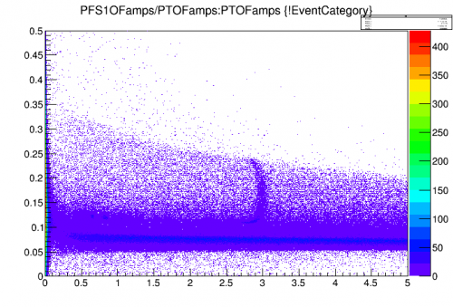 | 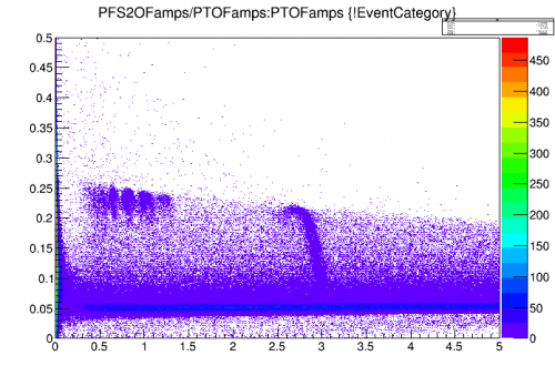 |
From these partition cuts its easy to see that the Am source must be near side two of the detector since that is where the higher partition and higher density regions appear for the lower Am lines. The 60 kev line is more spread throughout the detector. The Am can still be seen in the PFS1 Partition from the blue regions of data near the low band.
The calibration cut used and that which is used for the side 2 data is TCut chifs2=“PFS2OFamps/PTOFamps>0.15”, the calibration cut and that which is used for the side 1 data is TCut chifs1=“PFS1OFamps/PTOFamps>0.1”
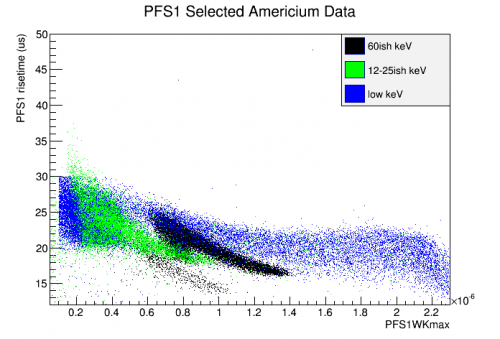
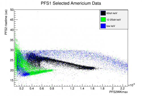
From here I went and plotted pulse risetime vs. amplitude for each side of PF with different primary channels, the resulting plots can be seen below.
| PFS1 Primary, PFS1 | PFS1 Primary, PFS2 |
|---|---|
 |  |
| PFS2 Primary, PFS1 | PFS2 Primary, PFS2 |
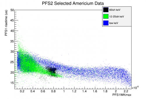 | 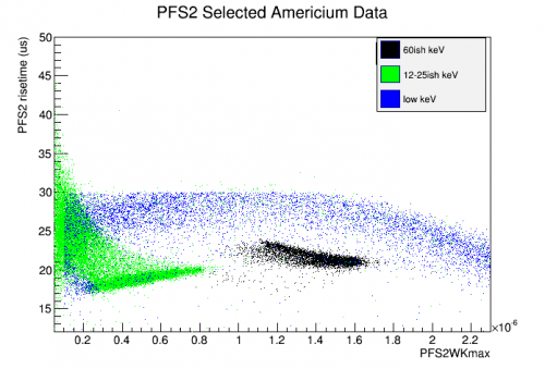 |
The interesting part about these plots shows up more heavily in the PFS2 primary channel data than the PFS1 primary. For PFS1 primary, the events are very spread out and cover a wider range of amplitudes and rise times than the PFS2 primary channel data. Another interesting fact is that the rise time for the PFS2 primary data with PFS2 plotted shows that high density region with low rise time once again where as the other data doesn't have the same feature. When the current primary channel is chosen and plotted the events for Am are more concentrated and in any other channel they are more spread. This might be compared with channel timing information to create a timing-independent z-position parameter based on energy and rise time alone. Which should still hold in the HV setting format.
II. Americium Depth From NIST and Side Partitioning
According to NIST X-Ray and attenuation coefficients we assume the use of the Beer-Lambert Law: I/I_0 = exp[(-(u/p)x] where the quantity u/p is the Mass Attenuation coefficient for in units of cm^2/g and x is a mass thickness given by x = pt in units of g/cm^2. Using the above relation I calculated the expected penetration depths for the Americium peaks using the NIST table for Silicon, and the Density of 2.32 g*cm^-3 for Silicon. The results are summarized in in Table II.1. The values of x and t are calculated from Beer-Lambert Law with a relative intensity of 10% initial intensity corresponding an equivalent drop in expected event rate and the penetration percentage comes from using a detector thickness of 30 mm.
| Table II.1: Expected Americium Depths | ||||
|---|---|---|---|---|
| Energy (KeV) | u/p (cm*cm/g) | x = pt (g/cm/cm) | t = x/p (mm) | % of detector penetration (%) |
| 10 | 3.389e1 | 0.068 | 0.293 | 0.98 |
| 15 | 1.034e1 | 0.223 | 0.960 | 3.20 |
| 20 | 4.464 | 0.516 | 2.223 | 7.41 |
| 60 | 3.201e-1 | 7.180 | 30.94 | 100 |
From the above, the Silicon is effectively transparent to the 60 keV peak and it should be seen throughout the detector while the other lines are much shallower with the 20 keV peak penetrating only 7% into the detector.
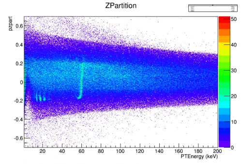
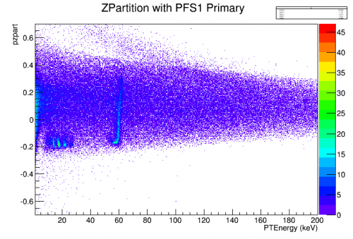
The next step is to create a side partitioning plot. This was done by using the following alias:
pzpart = (P*S1OFampsbal-P*S2OFampsbal)/(P*S1OFampsbal+P*S2OFampsbal)
Using this, I created to separate partitionings, one where I include all working and symmetric channels (with respect to PF) on both sides, and one where I include only the central channels in side partitioning. The working channels chosen where PF, PA, and PE for both sides. PB, PC, and PD where dead on side two of the detector. I should note that selecting a cut on PFS1 or PFS2 is degenerate for the location of the cut that I applied. In addition to the channel partition cut, I included a randoms cut and a set of energy cuts to take off extremely low energy events (E < 1) and to take off high energy events (E > 210) in order to discern an actual structure in the z partition.
| Z Partition of Si Americium Data, All Working Channels, PF selected | Z Partition of Si Americium Data, All Working Channels, None selected |
|---|---|
 |  |
| Z Partition of Si Americium Data, Only PF, PF selected | Z Partition of Si Americium Data, Only PF, None selected |
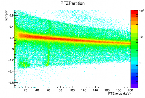 | 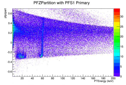 |
From the above plots and using the NIST information a depth representation can be constructed using the different partition methods. The table below summarizes possible depth values. These were obtained from using the event status bar and finding the difference between points for each energy.
| Table II.2 Depth values for Partitions | |||
|---|---|---|---|
| Energy | ZPartition | PFZParition | Real Distance (mm) |
| 60 | 0.5 | 2.53 | 30 |
| 20 | 0.12 | 0.2 | 2.223 |
| 15 | 0.12 | 0.2 | 0.960 |
It appears that this alone is not a good predictor of depth with a small resolution. The 20 and 15 keV peaks (corresponding to the 17.7 and 13.8 keV gammas) are basically indistinguishable using the partitions used. We effectively get two data points to fit these rates to an exponential which is not enough to get a correct estimate of depth. Either the ability to measure more peaks effectively (with more quality cuts used for control) or a different method such as relative timings between the side channels could lead to a more conclusive and hopefully interesting depth characterization for the these calibration lines.
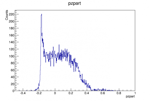
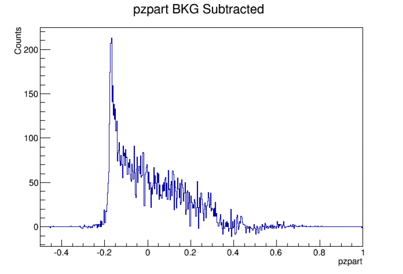
Using the data available I created a CDF of the measured data to compare to the cdf of the predicted (which is just the integral of the Beer-Lambert law with respect to x). I first selected out a range around the 60 keV peak and plotted zpart as a 1 dimensional histogram. I then cut out a small area of the same size directly next to the 60 keV peak for background to subtract off. I then integrated this histogram and normalized it to make the CDF for the measured data.
| PZpart 60 keV | PZpart BKG |
|---|---|
 | 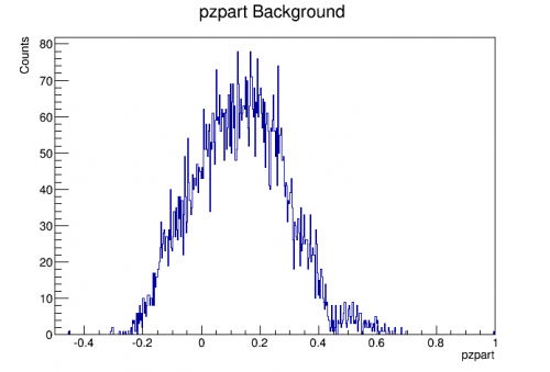 |
PZpart BKG was then subtracted from PZpart 60 keV to create the background subtracted figure.
| PZPart BKG Sub |
|---|
 |
This figure is then integrated piece-wise from 0 to each bin and the value of the integral is plotted as the ECDF below. I have included the theoretical CDF here as well for reference.
| PZPart ECDF | Theoretical CDF |
|---|---|
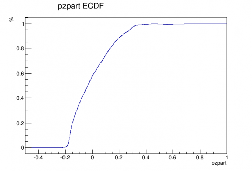 | 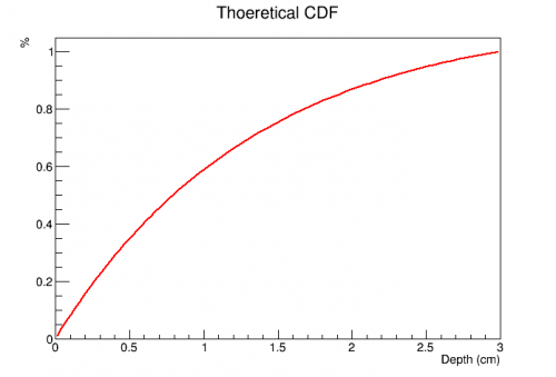 |
All the above figures are roughly what we expect. The background subtracted 60 keV spectrum is exponential in shape and the cdf appears to go as one minus the exponential. The next step is to map this expected value to a theoretical version of the depth. This is done by first normalizing the Beer-Lambert law to the max depth of the detector. The normalization factor comes to 0.359. Once we have a normalized spectrum we need to integrate this PDF from 0 to x to get theoretically predicted CDF. Integrating the beer lambert law, plugging in constants, and solving for t (the depth) gives:
t = -13.4*ln((1.12-cdf)/1.12) mm.
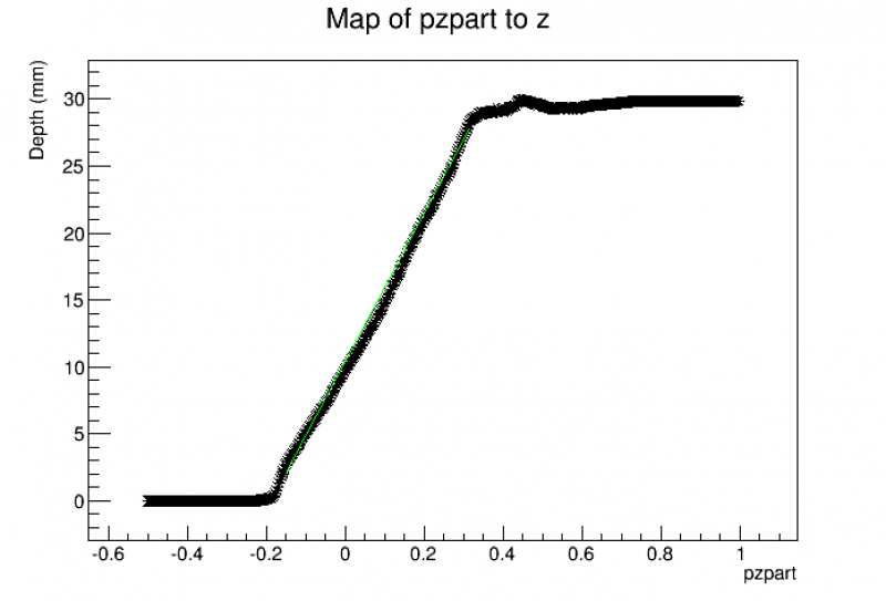
This equation was used to calculate the depth from the ECDF histogram above by using the percentages of the ECDF and mapping them directly to the predicted z depth. This was then plotted vs. pzpart and gave the following:
| PZPart Map |
|---|
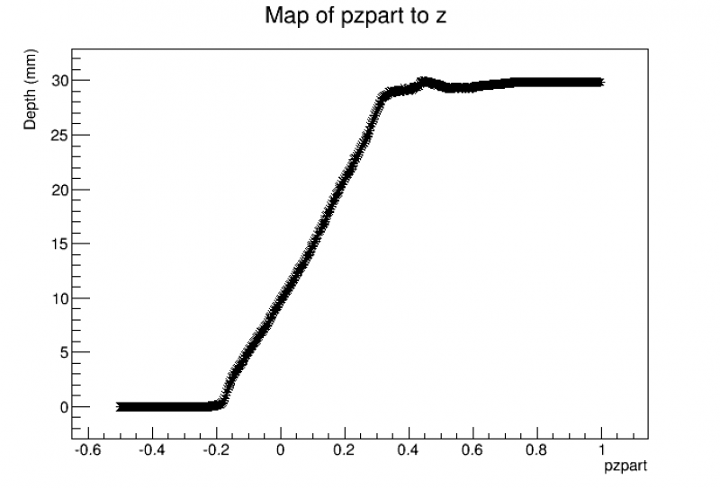 |
This plot trends as expected. the depth maxes out at 30 mm (the depth of the detector) and the values of pzpart follow what is expected from the 1D pzpart 60 keV histogram above. The most interesting thing about this is how linear the function of pzpart maps to real dimensions. It would be interesting to see if this continues to trend for the other versions of the map. There are also two areas where the mapping changes at pzpart of -0.2 which is near the surface of side 2 (where the Americium source is located) and near the the top of the detector depth where the slope of the line changes. The slope actually increases near the bottom surface where the Americium is indicating that the partition value is more sensitive near the leading edge of the detector than it is in the bulk or near the far surface. My guess as to why this is would be the types of phonons produced near the surface. 60 keV is a large energy scale compared to what is required to liberate electron hole pairs in Si (3.8 eV) This will produce a large fraction of high energy phonons as well as electron-hole pairs. These high energy phonons propagate quasi-diffusively at first before down converting into ballistic phonons. Near surface events should preferentially absorb the diffusive phonons due to a large number of interactions with the edge of the detector prior to full down conversion. This heightened rate fall off rather rapidly as the phonons tend to mostly ballistic by the time of first interaction with the detector surface and causes the abrupt change. The curved tail in the 60 keV line could hold more information about this and should be further explored.
I fit the linear region of the PZPart Map with a line by hand. The equation of best fit is as follows and is plotted below.
z=55.5*pzpart+10.47
| PZPart Map Fitted |
|---|
 |
PFZPartition Map
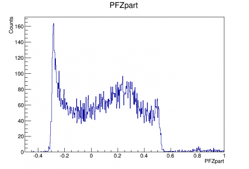
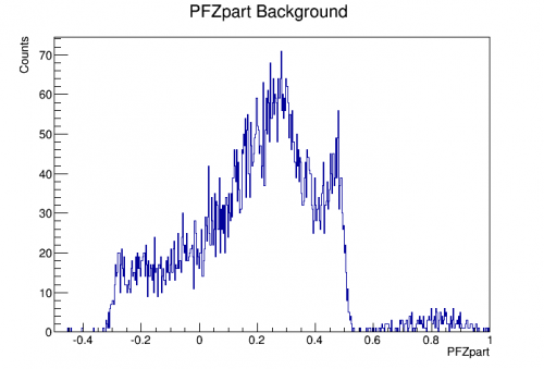
Let's try and do the same thing above but now using the PFZpartition alias. This alias was created as (s1-s2)/(s1+s2) or ONLY the central PF channel. This should hopefully give a cleaner signal dominated by the Americium and possibly a better fit quantity than what pzpart gives. The mapping will begin with 60 keV using the same cuts for the energy and background spectrums.
Using the same process outlined above the following is obtained:
| PFZpart | PFZpart Background |
|---|---|
 |  |
These are again subtracted to give the background subtracted spectrum.
| PFZpart BKG Subtracted |
|---|
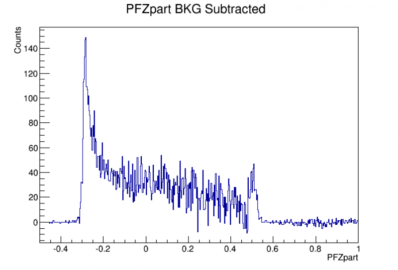 |
Integrating this bin by bin to create the ECDF which is plotted next to the same theoretical figure from above.
| PFZpart ECDF | Theoretical CDF |
|---|---|
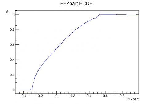 | |
These were then mapped to each other exactly as the above was done giving the following map.
| PFZpart Map |
|---|
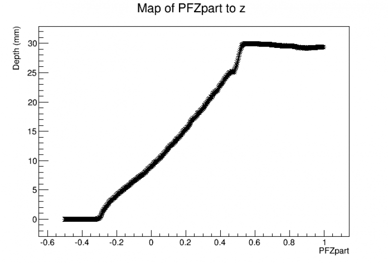 |
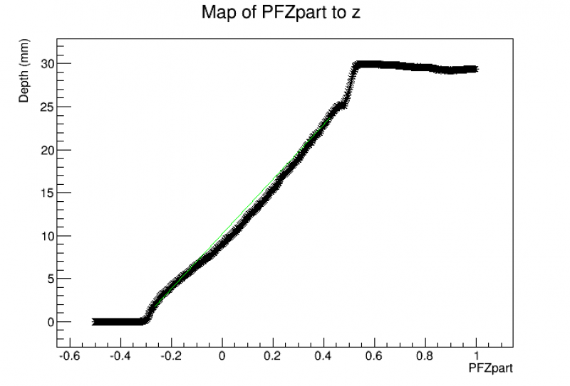
This figure was fit again with a line by hand, though this one is not as obviously linear. There are more slope changes and portions where it isn't quite linear but the best fit I could find by hand corresponds to
z=31.8*PFZpart + 10.2
Interestingly this has a rather different slope than the above mapping but the intercepts are very similar. I wonder if there is anything of interest there… The best fit is plotted below.
| PFZpart Map Fit |
|---|
 |
Curl Investigation
There are multiple sources of evidence for something odd happening with the energies near the surface of the detector, especially on side 2 near the Am source. The 60 keV has a large area of curl down to smaller energy, in addition, the lower energy lines appear to be mixed with lines with smaller penetration appearing higher in energy than those with lower penetration. This is a bit of mystery so I did a deep dive into pulse shape quantities on and near those surfaces. As it turns out, most of the pulse shape quantities don't show anything interesting, but the rise time, particularly for events near side 2 collected in energy on side 1, there is a clear discrepancy. The following plots were made using cuts to select either just the curl, the nearby 60 keV line, or back ground. These are plotted on the same figure for comparison.
| Pulse Height | |
|---|---|
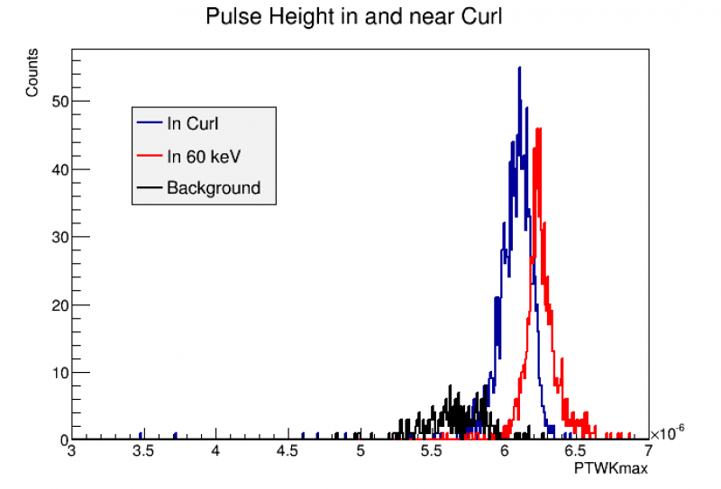 |
The pulse heigh in and around the curl seems to be energy dependent, which makes since the calibration should also be dependent on height as it depends on the OF fit. This shows that the overall height and possible energy of events in the curl are in fact lower energy than the 60 keV or, at the very least, have worse collection. It is important to note that this is constructed from the PT quantitiy so all channels are included here.
| Pulse Width |
|---|
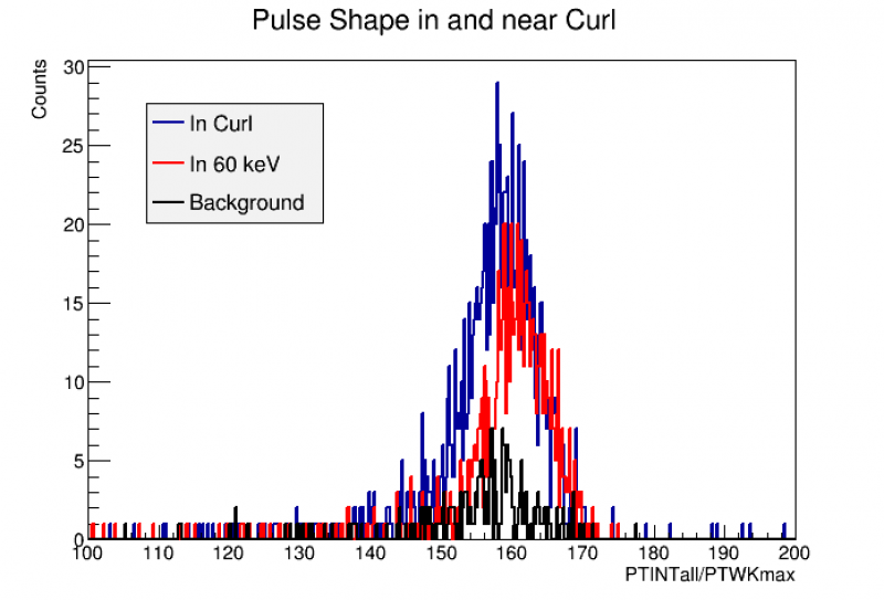 |
This figure is produced from PTINTall/PTWKmax which effectively is the area of the pulse divided by the height which should give the effective width. There appears to be little difference between the width of the different species of events looked at other than the number of events which is simply an artifact of the cut.
| Pulse Risetime Side 2 | Pulse Risetime Side 1 |
|---|---|
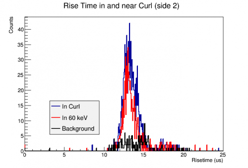 | 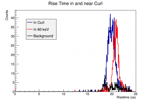 |
Here is where we see the first interesting difference. Lookin at the side of the detector closest to the event, there appears to be no difference in rise time of the three populations, though this makes sense due to the proximity to the surface, but, it appears there is a distinct difference when moving to the opposite face of the detector. In particulart, the 60 keV line has a decidely large rise time than that of the curl. The question then becomes why? A first thought would be due to some surface effects, especially if events in the curl are closer to the surface than those in the 60 keV line itself, but that seems somewhat unlikely since there are no effects of readout on that surface. It is also important to note that this is risetime only in the central channel, it would be interesting to see how risetime behaves in other channels to see if this effect persists or not. Another possible answer could be a difference in collection effeciency on the sides of the detector but one would assume both sides to be affected and not just the side closest to the Am source. This needs to e examined further but I'm sure what my best course of action is from here.