Table of Contents
Run 12
Summary
Setup
| Table 1: Run 12 setup | ||
|---|---|---|
| Detector | G42 | |
| Tower | T1 | |
| DIB | 1 | 2 |
| Face | 5 | 2 |
| Side coax | ZB1-1-9 | ZB1-1-6 |
| SQUET | ZC70 | ZC23 |
| Stripline | #20 | #19 |
| Readout | DCRCv3 | |
Tower level continuity checks can be found here (run diary: 2011/04/23). A complete record of electrical checks can be found here here (run diary: 2011/04/26).
There are two Am-241 sources above side 2 (ie. side with DIB2 Qi & Qo channels), installed within the 3“ source holder we use for oZIPs. One source lies in the centre of a phonon channel. The other lies to the side of another phonon channel, just within its boundaries.
Additional Neutron Shielding
Prior to cool down, polyethylene sheets have been installed within the IVC and main bath as shown in Figure 1. Within the IVC, a cylinder of length 1.5” and diameter 4“ has been fastened to the top of the 30 mK stage. The tower comfortably slots in below it. A further nine 1” diameter polyethylene sheets have been placed around the top of the IVC. These will supplement the external neutron shield.
| Figure 1: Polyethylene sheets fastened to top of 30 mK stage within can (left); Polyethylene sheets around top of IVC (right). | |
|---|---|
 |  |
DAQ Issues
We received a new version of the DAQ code from Jeter to write iZIP format data files. Currently we have been collecting and analysing oZIP format data, which would have meant treating each DIB as a separate detector. There were some teething problems, but these have been resolved. Nothing to write home about.
Cryogenic Issues
We have been plagued by random losses in base temperature this run. The fridge has been very temperamental. Sometimes she works beautifully and consumes hardly any helium, and at other times she goes insane and gorges herself. We suspected a blockage was causing the random rise in base temperature. If this was the cause, it has magically cleared itself as far as we can tell. Although the fridge still occasionally struggles to reach a base temperature of 53 mK after a long detector flash, but this is easily solved by adjusting the still heater.
We have had problems with the 1 K pot in the past. A thorough clean would be prudent before the next run.
Searching for Neutralisation
Changes to Data Taking Procedure
We usually use a trace length of 1.6384 ms and trigger delay of 400 μs for oZIPs. Due to the larger size of these crystals, we noticed a higher background which led to increased pile-up. In an effort to improve efficiency, the trace length and trigger delay have been reduced to 0.4096 ms and 100 μs respectively. This is adequate for studying neutralisation. It has paid dividends, as the 356 keV peak from Ba-133 is clearly visible since switching.
Some flashing parameters have also changed. These are outlined in Table 2.
| Table 2: Old vs. New Flashing Parameters. | ||
|---|---|---|
| Parameter | Old Setting | New Setting |
| LED | 1 | 1 & 2 |
| Current | 0.6 mA | 0.6 mA |
| Flash on time | 100 μs | 100 μs |
| Flash off time | 2.5 ms | 5.0 ms |
Data has been taken during overnight runs using the autorun feature of the DAQ. Typically, 60 minutes of data are taken before flashing and cool down. This procedure is repeated until the DAQ spits out an error or we get tired. A new data series is started after every iteration.
Qi & Qo on DIB1 are always biased at -2.5 V (ie. side 1 always collects holes). Of course, the reverse is true for the opposite side.
Outline of Analysis Procedure & Cuts
| Table 3: Outline of Cuts. | ||
|---|---|---|
| Cut | Description | Value |
| Q inner | Gaussian fit to peak at Qpart ( (QIS*OFvolts-QOS*OFvolts)/(QIS*OFvolts+QOS*OFvolts) ) ≈ 1. | Qpart = Mean ± 3σ |
| χ² | Gaussians fit to slices projected along y-axis in χ² vs. Qsum (QIS*OFvolts+QOS*OFvolts) distributions, and quadratic polynomial fit to the (Mean + 5σ) histogram that arises. | Qsum < quadratic polynomial. |
| Bulk | Gaussians fit to slices projected along the y-axis in Side 1 vs. Side 2 Qsum distributions after above cuts. Straight lines fit to (Mean + 3σ) & (Mean - 3σ) histograms that arise. | Event lies within these lines. |
A quick outline of cuts is given in Table 3 and illustrated in Figures 2 & 3. The resultant Qsum histograms and Qsum vs. Time scatter plots after these cuts are shown in Figure 4.
It is clear from Figure 2 that there is little crosstalk between Qi and Qo on either side, making a correction unecessary.
| Figure 2: Illustration of basic cuts (Q inner & χ²) with data series 07110510_1834. |
|---|
 |
| Figure 3: Illustration of bulk cut with data series 07110510_1834. |
|---|
 |
| Figure 4: Resultant Qsum histograms and Qsum vs. Time scatter plots after all cuts for data series 07110510_1834. |
|---|
 |
 |
With reference to Figure 4, the Ba-133 peak is well-defined on Side 1 (ie. the side that collects holes). After speaking with Bruno, it appears that the negatively biased side is used in charge studies for this reason. Therefore, we shall only consider Side 1 when investigating neutralisation.
First Decent iZIP Data Taken with K100
After speaking with Todd, it appears that we might be flashing for an unecessarily long time. Berkeley typically flash for a total of 1-2 s, and cool down for 5 minutes. After flashing for 6 s, we determined that we require 12 minutes to return to base temperature. Therefore we used these parameters for our first overnight data run. The DAQ output a “memory full” error 44 minutes into the fifth iteration.
Qsum and Qsum vs. Time distributions for one of the data series collected is shown in Figure 5 at 15-, 30- & minute time intervals. Distributions from the other data sets taken during this run can be found here (run diary: 2011/05/12).
| Figure 5: Qsum and Qsum vs. Time distributions for third data series 07110512_0218 at 15-, 30- & 60-minute time intervals. |
|---|
 |
 |
 |
From the Qsum vs. Time distributions, it can be inferred that we lose neutralisation after approximately 15 minutes. Armed with this information, we can compare the 356 keV peak positions for each run in Figure 6.
| Figure 6: Qsum spectra for files taken on 2011/05/12. |
|---|
 |
Surprisingly, the peaks do not line up: a mean position of 0.000517 ± 0.000044 (8.5%) units is obtained, together with a standard deviation of 0.000098 (19% of mean) units. At first glance this could be a result of neutralisation. However, on closer inspection it looks more like a gain problem. This is more evident when the peaks are scaled, as shown in Figure 7. The background spectra lie on top of each other, as one would expect. Additionally, the 356 keV peak is well-defined in each data series.
| Figure 7: Qsum spectra for files taken on 2011/05/12, scaled to 356 keV peak position from 07110512_0105. |
|---|
 |
After 24-Hour Bake
Although it is unlikely to be a neutralisation problem, it would be unwise to dismiss this possibility. We placed the Ba-133 source as close as possible to the detector, and baked & flashed it for 24 hours before taking our next overnight data run. This time the DAQ lasted an extra 2 minutes, crashing 46 minutes into the fifth data set. The resultant Qsum spectra are shown in Figure 8, and individual distributions are given here (run diary: 2011/05/14).
| Figure 8: Qsum spectra for files taken on 2011/05/14. |
|---|
 |
At first glance, the results look better. However, the first data series has not been plotted. The Qsum and Qsum vs. Time distributions for this series are shown in Figure 9.
| Figure 9: Qsum and Qsum vs. Time distributions for first data series 07110513_2327 during the first 15 minutes. |
|---|
 |
This does not make too much sense. The first data set was taken after the detector was left to cool down for 3 hours. If the detector was not grounded properly, this should be the worst data series (ie. should yield the lowest energy) due to charge build-up while idle. If the detector was sufficiently grounded, this data series should look identical to the rest. What's going on?
A mean peak position of 0.000703 ± 0.000034 (5%) units is obtained, together with a standard deviation of 0.000077 (11% of mean) units.
Increase Total Flash Time to 20 Minutes
To try to isolate the problem, we returned to our old system of flashing the detector for 20 minutes rather than 6 s in attempt to remove some unknowns. Another overnight data run was undertaken, and again the DAQ crashed 46 minutes into the fifth data series. The resultant Qsum spectra are shown in Figure 10. Qsum spectra for data sets taken during this run over 15-, 30- & 60-minute time intervals are given here (run diary: 2011/05/17).
| Figure 10: Qsum spectra for files taken on 2011/05/17. |
|---|
 |
A mean peak position of 0.000670 ± 0.000018 (2.7%) units and a standard deviation of 0.000040 (6.0% of mean) units is obtained. This is better, but still awful.
Why we are Adamant that we can Neutralise iZIPs
This section could also be titled 'Why we are Sure this is a Gain Problem'. What does bad neutralisation look like? To investigate this, we can plot Qsum spectra for the first and final 15 minutes for a few data series. These are shown in Figures 11, 12 & 13.
A clear peak at a high energy is visible in Figures 12 & 13 during the first quarter-hour, each taken from data sets taken on different days. Once neutralisation is lost, the peak cannot be made out, let alone fitted to. It merges into the background. This is different behaviour from what we see above. In each data set, the 356 keV peak is clearly visible and significant during the first 15 minutes.
| Figure 11: Qsum spectra during first and final 15 minutes for data series 07110512_0102. |
|---|
 |
| Figure 12: Qsum spectra during first and final 15 minutes for data series 07110514_0313. |
|---|
 |
To drive the point home, we can take a look at the data set that yielded the lowest position for this peak in Figure 13. Even here, the 356 keV peak is clearly visible above the background during the first 15 minutes, and is missing during the last.
| Figure 13: Qsum spectra during first and final 15 minutes for data series 07110512_0330. |
|---|
 |
Armed with this knowledge, it is possible that flashing the detector for 6 s is adequate.
Performance of Old DAQ
There are 5 possible places where this problem could lie: the crystal; the DCRC boards; the DAQ software; the reduction code; or me. To try to eradicate some of these possibilities, we turned to the old DAQ we ran last run with the 100 mm crystal. Data is taken in oZIP format. As we are not looking at side 2, this does not prove to be an issue. It does however mean that we cannot implement a bulk cut. This time we got tired of the taking data and stopped the DAQ after the sixth data series. Qsum distributions for all data sets taken are given here (run diary: 2011/05/19). A typical first 15-minute spectrum is shown in Figure 14.
| Figure 14: Qsum and Qsum vs. Time distributions for third data series 07110519_0600 over the first 15 minutes. |
|---|
 |
With reference to Table 4, it appears that taking data in the oZIP format provides a more consistent result. It appears that this is either an issue with the DAQ code or the processing of iZIP data with cdmsbats.
| Table 4: Comparison of Mean and Standard Deviation values between different data series. | |||
|---|---|---|---|
| Date | Description | Mean [arbitrary units] | Standard Deviation [arbitrary units] |
| 2011/05/12 | Take data for 60 mins, flash detector for 6 s, cool down for 12 mins. | 0.000517 ± 0.000044 (8.5%) | 0.000098 (19% of mean) |
| 2011/05/14 | Bake detector. Take data for 60 mins, flash detector for 6 s, cool down for 15 mins. | 0.000703 ± 0.000034 (5%) | 0.000077 (11% of mean) |
| 2011/05/17 | Take data for 60 mins, flash detector for 20 mins, cool down for 60 mins. | 0.000670 ± 0.000018 (2.7%) | 0.000040 (6.0% of mean) |
| 2011/05/19 | Old DAQ. Take data for 60 mins, flash detector for 20 mins, cool down for 60 mins. | 0.01684 ± 0.00007 (0.4%) | 0.00018 (1.1% of mean) |
2-Hour Ba-133 Data Series
With the above in mind, we used the old DAQ to acquire our remaining data series. To cross-check our performance with Berkeley, we took 2-hour long runs exposing the detector to a Ba-133 source. The phonon channels were tuned and locked for these runs, the trace length was increased to 3.2768 ms, and the trigger was set at 18 phonon ADC bins (OR trigger). In an effort to reduce pile-up, the Ba-133 source was moved further back (6“ below top of mu-metal shield).
| Figure 15: Qsum from data series 07110525_1928 (3.2768 ms trace length, Ba-133, phonon and charge signals). |
|---|
 |
| Figure 16: Phonon Response. Outer phonon channels A1 & A2 are not included. |
|---|
 |
| Figure 17: Box plots after cuts (top), and when Qsum on Side 2 lies between 50 keV and 80 keV. | |
|---|---|
 |
|
 |  |
 |  |
| Figure 18: Box plots after cuts (left), and when Qsum on Side 2 lies between 50 keV and 80 keV. |
|---|
 |
 |
 |
| Figure 19: Relative Phonon Calibration (left) and Yield vs. Phonon Energy (right). Luke phonons are not taken into account. |
|---|
 |
| Figure 20: Qzpart (left) and Yield (right) as a function of time. |
|---|
 |
6-Hour Ba-133 Data Series
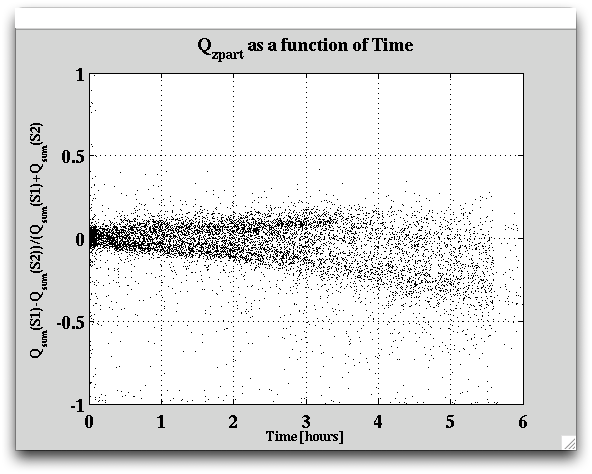
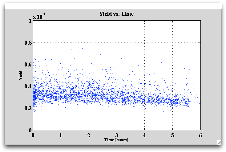
To determine how long it actually takes to see degredation in the yield and Qzpart, a 6-hour long data series was recorded.
| Figure 21: Qzpart as a function of time. |
|---|
 |
| Figure 22: Yield as a function of time. |
|---|
 |
Flipping Bias every 20 Minutes
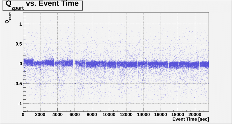
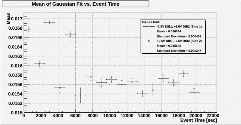
To see whether reversing the bias had any positive effect on neutralisation loss, we took a number of data series where the bias was flipped every 20 minutes with no flashing in between.
| Figure 23: Qzpart as a function of time. |
|---|
 |
| Figure 24: Mean of Gaussian fits to 356 keV peak as a function of time. |
|---|
 |
Fall and Rise Time Constants
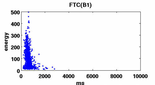
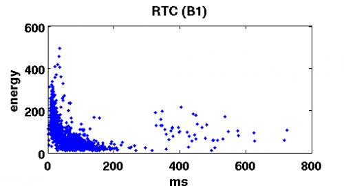
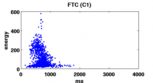
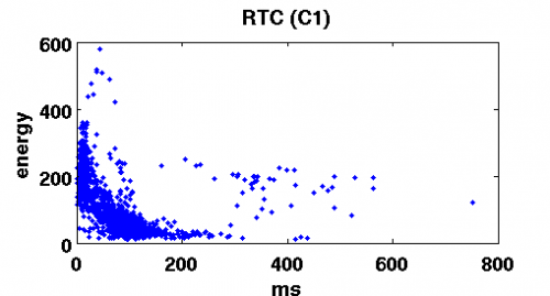
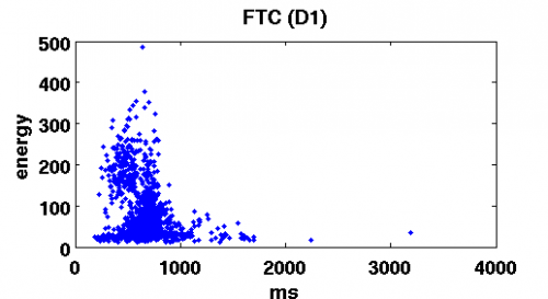
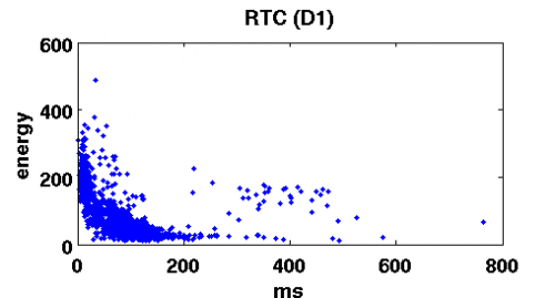
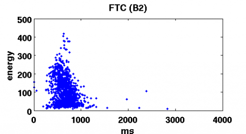
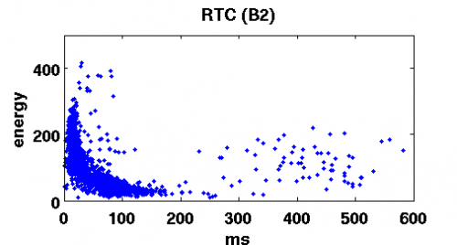
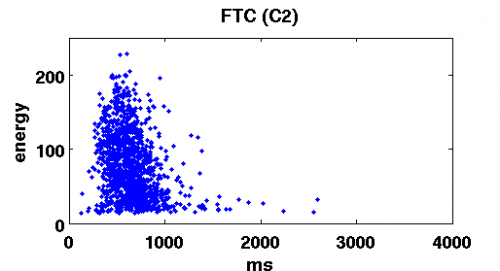
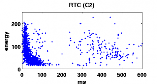
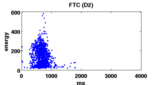
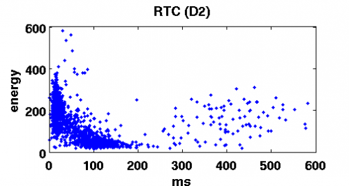
Graphs clearly indicate independence of the FTC on energy and possibly an inverse relation of RTC and phonon energy
| Fall time constant | Rise time constant |
|---|---|
 |  |
 |  |
 |  |
 |  |
 |  |
 |  |