Phonon Collection Efficiency for S104
Phonon collection efficiency is an interesting detector property, but it's a side topic for analysis - it's not relevant to the (n,gamma) NR calibration.
The basic idea to calculate phonon collection efficiency is to compare the amount of energy absorbed in the TESs to the total amount of phonon energy in an event. The former you get from an absolute calibration of the detector, and the latter you get from an energy calibration using calibration lines, plus any NTL gain. It's easiest to use 0-volt data so you don't have to deal with uncertainty in the NTL gain. (Although if there's a difference in PCE for NTL phonons versus other phonons you'd want to try to do PCE calculations for biased data too.)
Early in Run76 we took three 2-sided data series (necessarily at 0-V bias). A nice feature of these series is that the source was at different locations, so we can see whether the PCE calculation depends on the position of the calibration source.
This first code block loads one of the three series:
// first three source-position data series
char* sers[3] = {"07220330_1639", "07220405_1646", "07220406_1720"}
//
// choose one series below to load into data (0, 1, or 2)
int s = 2
//
gStyle->SetOptStat(0)
char* ser = sers[s]
TChain *e = new TChain("rqDir/eventTree")
TChain *z = new TChain("rqDir/zip1")
int nsparse = 1
char* datapath ="/data/chocula/fritts/data/k100proc/midasrq/byseries/"
e->Add(Form("%s/%s/umn*root",datapath,ser));
z->Add(Form("%s/%s/umn*root",datapath,ser));
z->AddFriend(e)
TCut crand = "EventCategory"
The next code block is the absolute calibration. This is done channel by channel, and at the end they are summed to give the total absorbed energy in an event.
This is based on the integral amplitudes. We convert a raw integral to V*s units, then to A*s units using the gains in the feedback circuit. Then convert that to W*s using dP/dI, which is calculated from IbIs data. I made a convenient choice with this run to choose a uniform value for dP/dI then tune all the QET biases to that value. That makes the channels automatically balanced (in theory) and it makes the PCE calculation a lot easier.
Shown here is the linear approximation for the absorbed energy. If the change in current in an event is small compared to the bias current, the linear approximation is pretty good. It's possible though to add a non-linear correction. This is more necessary for high-amplitude events (so it would be more important in biased data). If we get an energy dependence in our calculated PCE we should trust the value at lower energies more than higher energies.
//////////////////////////
// Absolute Calibration
char* chanIDs[12] = {"PAS1", "PBS1", "PCS1", "PDS1", "PES1", "PFS1", "PAS2", "PBS2", "PCS2", "PDS2", "PES2", "PFS2"}
float gdcrc = 2; float gdriver = 1;
//
float qetbias_muamp[12] = {229.5, 241.7, 255.8, 258.9, 260.8, 287.1, 170.3, 178.2, 172.5, 209.4, 216.1, 175.5}
// note: above values are not necessary because all channels were tuned to a specific dP/dI
//
float adcPERvolt = 6553.6, secPERsample = 8e-7;
float rfb_ohms = 1233; float gloop = 10.5; // rfb is the feedback resistor in ohms
float rshunt_ohm = 8.e-3
float joulePERkev = 1.60218e-16
// New courtesy of Nick: conversion for the INTall RQs to convert them to ADC*sample units, using the "norm" RQ:
for(int c=0;c<12;c++)z->SetAlias(Form("%srawINT",chanIDs[c]),Form("%sINTall*%snorm",chanIDs[c],chanIDs[c]))
// convert from units ADC*samples to V*s
for(int c=0;c<12;c++)z->SetAlias(Form("%sINT_Vs",chanIDs[c]),Form("%srawINT/%f*%e",chanIDs[c],adcPERvolt,secPERsample))
// convert from V*s to coulombs (amount of charge through TES). need to know gains.
float rgain_ohm = rfb_ohms*gloop*gdcrc*gdriver
for(int c=0;c<12;c++)z->SetAlias(Form("%sINT_C",chanIDs[c]),Form("%sINT_Vs/%f",chanIDs[c],rgain_ohm))
// calculate linear approximation of absorbed energy
float PoverIlin_volt = 1.0e-6 // set to the same value for each channel
for(int c=0;c<12;c++)z->SetAlias(Form("%seabs1_keV",chanIDs[c]),Form("%sINT_C*%e/%e",chanIDs[c],PoverIlin_volt,joulePERkev))
// get total absorbed energy per event, linear approx
//
z->SetAlias("PTOTeabs1_keV", "PAS1eabs1_keV+PBS1eabs1_keV+PCS1eabs1_keV+PDS1eabs1_keV+PES1eabs1_keV+PFS1eabs1_keV+PAS2eabs1_keV+PBS2eabs1_keV+PCS2eabs1_keV+PDS2eabs1_keV+PES2eabs1_keV+PFS2eabs1_keV")
//
//////////////////////////
Next we do the standard deposited-energy calibration of the OF amplitude using Am peaks. First we construct a cut to select Am events based on energy fraction, so it's easier to fit the peaks. In the example here I do this for the third series (s=2), leaving the cuts for the other two series blank for now. I fit the 14keV, 18keV, and 60keV lines, and also include (0,0), and construct a quadratic calibration function (though the calibration is pretty close to linear).
// electron-equivalent energy calibration
//
// use energy fraction in Am channel to make Am-selection cut for cal spectrum
// once you choose a threshold you can add the cut here:
TCut cam[3] = {"1", "1", "PES1OFamps/PTOFamps>0.16"}
// note: for s=0,s=1 PFS1OFamps is best for identifying Am events; for s=2 PES1OFamps is best
//
if(s<2)  z->Draw("PFS1OFamps/PTOFamps:PTOFamps>>hefe(300,0,3e-6,200,0,0.5)",!crand,"colz")
if(s==2) z->Draw("PES1OFamps/PTOFamps:PTOFamps>>hefe(300,0,3e-6,200,0,0.5)",!crand,"colz")
//
z->Draw("PTOFamps>>hamspec(200,0,3e-6",!crand+cam[s])
TGraph gcal
gcal.SetPoint(0,0,0)
if(s==2)hamspec->Fit("gaus","","",0.46e-6,0.52e-6)
gcal.SetPoint(1,hamspec->GetFunction("gaus")->GetParameter(1),13.95)
if(s==2)hamspec->Fit("gaus","","",0.595e-6,0.68e-6)
gcal.SetPoint(2,hamspec->GetFunction("gaus")->GetParameter(1),17.74)
if(s==2)hamspec->Fit("gaus","","",1.85e-6,2.10e-6)
gcal.SetPoint(3,hamspec->GetFunction("gaus")->GetParameter(1),59.54)
//
gcal.Draw("a*")
gcal.Fit("pol2")
// quadratic fit - but it's nearly linear!
z->SetAlias("ptof_keV",Form("%e+%e*PTOFamps+%e*PTOFamps*PTOFamps",gcal.GetFunction("pol2")->GetParameter(0),gcal.GetFunction("pol2")->GetParameter(1),gcal.GetFunction("pol2")->GetParameter(2)))
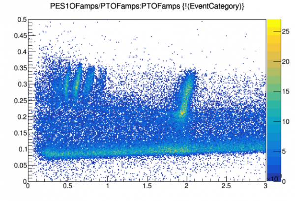 |
| Here we plot PES1OFamps/PTOFamps versus PTOFamps, because in this series PES1OFamps gets more of a share of the energy from Am events than the other channels. A minimum threshold of 0.16 is chosen to select Am events. |
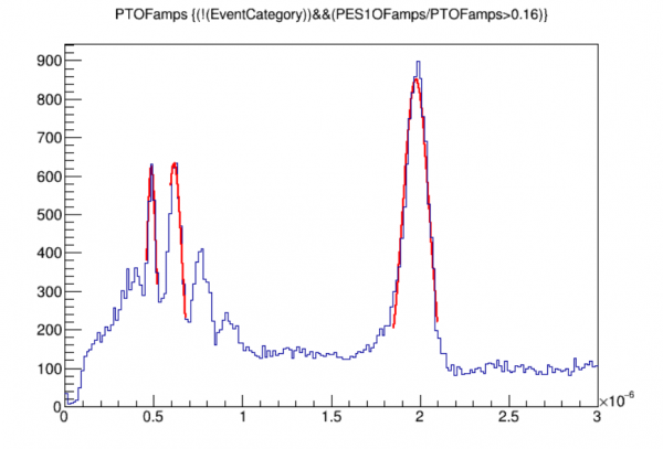 |
| Here we've drawn a spectrum in PTOFamps and fit three lines. NOTE: as mentioned before, for the 18keV line you should avoid the left side of the peak because there is a second line in the left shoulder of the 18keV peak. |
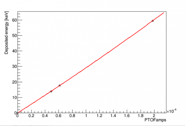 |
| A quadratic fit to the calibration points. (0,0) is included as a calibration point. Note the calibration is nearly linear. |
Now we have the absolute absorbed energy (based on integral amplitudes) and the calibrated deposited energy (based on OF amplitudes) for every event. Note that at 0V the deposited energy is the same as the total phonon energy. Next we define phonon collection efficiency, see if appears to depend on energy, and do some calculations:
z->SetAlias("pce","PTOTeabs1_keV/ptof_keV")
//z->Draw("pce:ptof_keV",!crand+"pce>0&&pce<1")
z->Draw("pce:ptof_keV>>hpcevewide(300,0,400,200,0,1)",!crand,"colz")
z->Draw("pce:ptof_keV>>hpceve(300,0,100,200,0,1)",!crand,"colz")
hpceve->SetTitle(";deposited energy [keV];phonon collection efficiency")
hpceve->Draw("colz")
//
z->Draw("pce>>hpcelo(100,0,1)",!crand+"ptof_keV>2&&ptof_keV<30")
hpcelo->Fit("gaus","","",0.25,0.6)
// FOR S=2: Mean         3.12987e-01   4.22180e-04   4.15169e-06  -1.75268e-01
//
z->Draw("pce>>hpcehi(100,0,1)",!crand+"ptof_keV>50&&ptof_keV<70")
hpcehi->Fit("gaus","","",0.25,0.6)
// FOR S=2: Mean         3.31448e-01   1.96954e-04   2.86876e-06   4.01206e-02
//
// wow - phonon collection efficiency around 32%
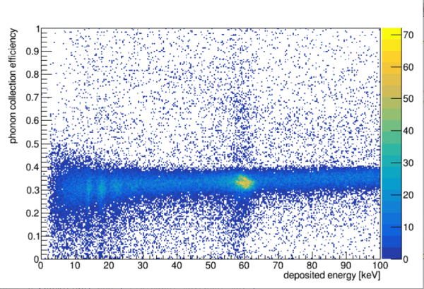 |
| Phonon collection efficiency versus energy. We cut the plot off at 100 keV since we really only trust the calibration out to 60 keV. |
This detector has the highest PCE we've ever measured: around 32%. Somewhat higher at 60 keV than at the lower energies (31.3% at low energy).
To Do:
- Repeat the Am selection, deposited energy calibration, and PCE plot and calculations for the first two series (s=0 and s=1). For these, S1PF is the best channel to use to set the Am-selection cut.
- No cuts have been applied except to remove randoms. The PCE versus energy plot would have fewer outliers if a chisquare cut were developed and applied. Not totally necessary.
- The PCE results for the three series should be compared. Differences between them would suggest a systematic uncertainty. Presumably an average value should be used to quote the detector's estimated PCE.
- If desired a nonlinear correction can be applied to the absolute calibration (see Matt for details).
Non-linear correction
The absolute calibration above is a linear approximation. For strong signals - i.e. when the change in current during a pulse is a significant fraction of the bias current - 2nd-order effects become important.
An approximation of the 2nd-order correction can be calculated with some knowledge of the pulse shape, which we have access to from the walk algorithm quantities. Details can be found in this dP/dI note and this linked nonlinear correction method note (login scdms, passord SoupR).
This code block gives the 2nd-order absolute calibration (after first calculating the first-order one):
//////////////////////////
// Second order corrected absolute calibration
// calculate approximate tau of pulse - a sort of pulse width
for(int c=0;c<12;c++)z->SetAlias(Form("%s_it",chanIDs[c]),Form("-20*%sWKr10+-5*%sWKr20+-10*%sWKr30+-10*%sWKr40+-10*%sWKr50+-10*%sWKr60+-10*%sWKr70+-10*%sWKr80+-10*%sWKr90+0*%sWKr100+10*%sWKf90+25*%sWKf80+20*%sWKf40+40*%sWKf20",chanIDs[c],chanIDs[c],chanIDs[c],chanIDs[c],chanIDs[c],chanIDs[c],chanIDs[c],chanIDs[c],chanIDs[c],chanIDs[c],chanIDs[c],chanIDs[c],chanIDs[c],chanIDs[c]))
//
for(int c=0;c<12;c++)z->SetAlias(Form("%s_i2t",chanIDs[c]),Form("-300*%sWKr10+-350*%sWKr20+-600*%sWKr30+-800*%sWKr40+-1000*%sWKr50+-1200*%sWKr60+-1400*%sWKr70+-1600*%sWKr80+-1800*%sWKr90+0*%sWKr100+1800*%sWKf90+3250*%sWKf80+2800*%sWKf40+1200*%sWKf20",chanIDs[c],chanIDs[c],chanIDs[c],chanIDs[c],chanIDs[c],chanIDs[c],chanIDs[c],chanIDs[c],chanIDs[c],chanIDs[c],chanIDs[c],chanIDs[c],chanIDs[c],chanIDs[c]))
//
for(int c=0;c<12;c++)z->SetAlias(Form("%s_tau_s",chanIDs[c]),Form("%s_it**2/%s_i2t",chanIDs[c],chanIDs[c]))
//
// calculate 2nd-order corrected dP/dI
float res_ratio = 1.5 // this is 1+Rpar/Rshunt. Best to estimate this for each channel from IbIs, this is an approximation instead.
for(int c=0;c<12;c++)z->SetAlias(Form("%s_PoverI2_volt",chanIDs[c]),Form("%e+%f*%e*%sINT_C/%s_tau_s",PoverIlin_volt,res_ratio,rshunt_ohm,chanIDs[c],chanIDs[c]))
// calculate 2nd-order corrected absorbed energy
for(int c=0;c<12;c++)z->SetAlias(Form("%seabs2_keV",chanIDs[c]),Form("%sINT_C*%s_PoverI2_volt/%e",chanIDs[c],chanIDs[c],joulePERkev))
// get total absorbed energy per event, 2nd-order corrected
z->SetAlias("PTOTeabs2_keV", "PAS1eabs2_keV+PBS1eabs2_keV+PCS1eabs2_keV+PDS1eabs2_keV+PES1eabs2_keV+PFS1eabs2_keV+PAS2eabs2_keV+PBS2eabs2_keV+PCS2eabs2_keV+PDS2eabs2_keV+PES2eabs2_keV+PFS2eabs2_keV")
//////////////////////////
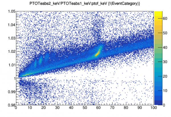
The plot below shows that the correction is less than 3% for event energies below 100 keV.
z->Draw("PTOTeabs2_keV/PTOTeabs1_keV:ptof_keV>>hcorrve(300,0,100,200,0.98,1.05)",!crand,"colz")
 |