Below are plots of the peak in Channel 4 versus time into the series.

Figure 1
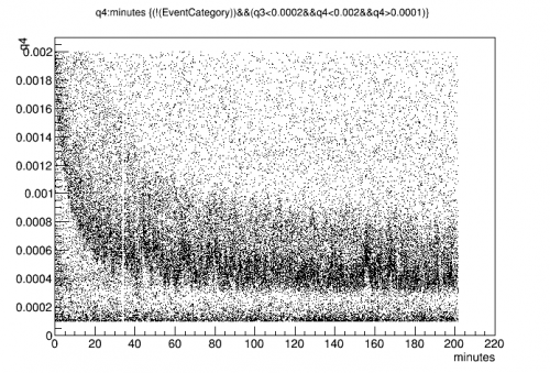	12 V	240 min after flash
The data started a few minutes after applying the bias, and a long time after the flash. The peak falls in the first several minutes to a baseline 0.0004 is the approximate “correct” position of the 60 keV line. It seems to be higher than this initially.

Figure 2
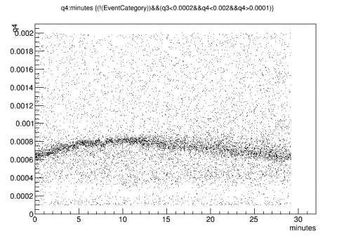	5 V	30 min after flash
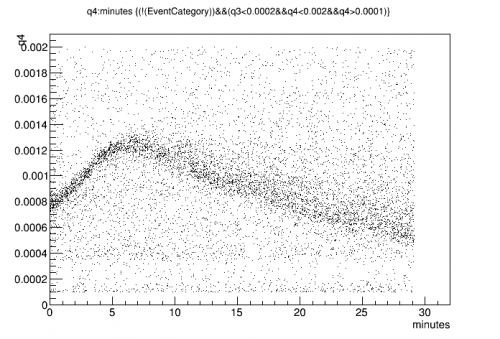	7 V	30 min after flash
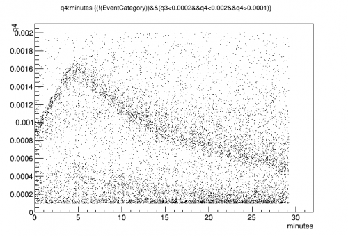	8 V	30 min after flash
	9 V	30 min after flash
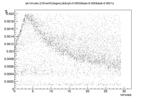
Above is data during a bias sweep. Data starts right after applying bias. The peak maximum is higher and sooner with higher bias.

Figure 3
	-3 V	30 min after flash
	-7 V	30 min after flash
	-11 V	30 min after flash
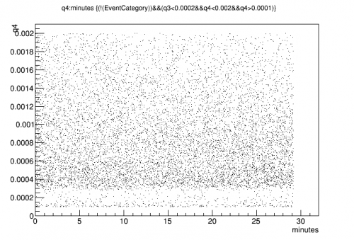
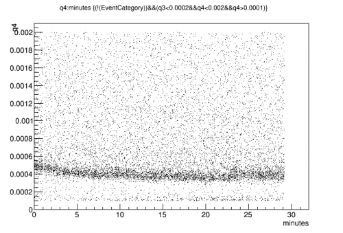
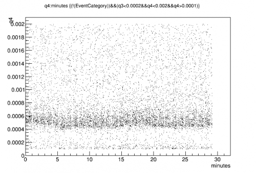
Above is data during a bias sweep, negative bias. Here the time-dependence is not seen or is much smaller than with positive bias.

Figure 4
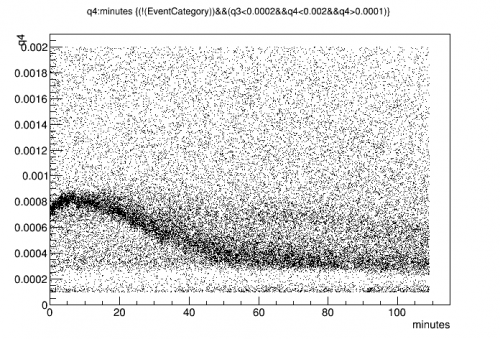	5 V	5 min after flash
This is data started right after a flash - the tower was still cooling Also temperature variations were applied during the series. The change in peak position seems independent of temperature. It seems to be a matter of time after bias.

Figure 5
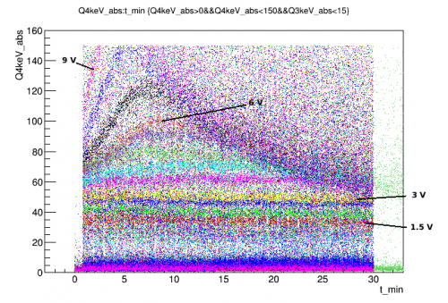Several of the above data sets overlayed. The y-scale is an absolute calibration to keV which includes detector gains and estimated capacitances based on R65 measurements.

Figure 6
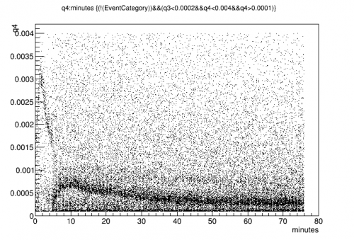Here we set the bias to 11 V for 6 minutes, then to 6 V attempt at a “prebias”

Figure 7
8 V
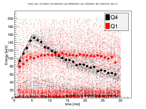A comparison of Q1 (outer) and Q4 (inner) signals vs time. In general, Q4 is more variable than Q1. Q2 and Q3 seem to be a mix of these two extremes.

Figure 8
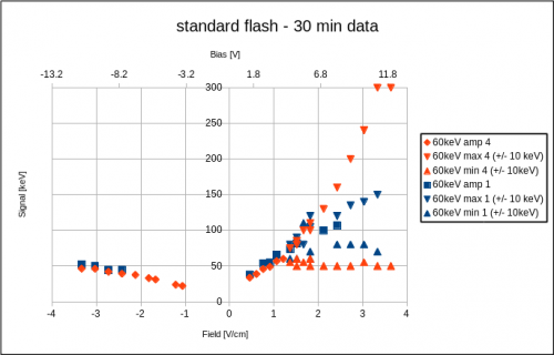Preliminary seagull plots of Q1 and Q4. At negative biases, there is little variation in 60 keV line position over time. At positive biases, the time-dependent hump appears at fields biases above 1.25 V/cm. Thereafter, the approximate range of the calibration line for the first 30 min is plotted. Q1 shows similar behavior as Q4 but with less spreading at high positive biases.

Figure 9
Q4 vs time after biasing. First series was after a standard ground and flash, subsequent series each had only 10min grounding in between.

Figure 10
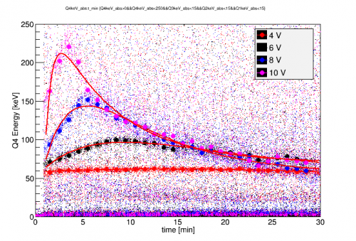Preliminary model fits to Q4 peak vs time. <m>Q_0</m> is the charge created by an event, C is the standard charge collection efficiency, A is an impact ionization efficiency, <m>\tau_{Imp}</m> is the lifetime of impact ionization site population, B is a strong trapping efficiency, and <m>\tau_{Trap}</m> is the strong trapping population lifetime.

Figure 11
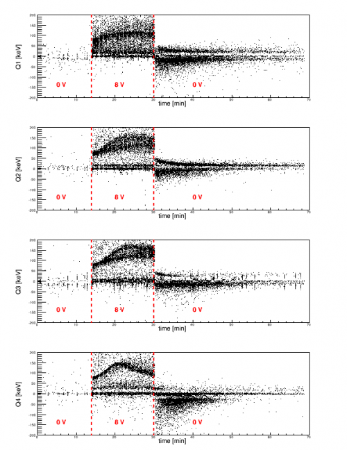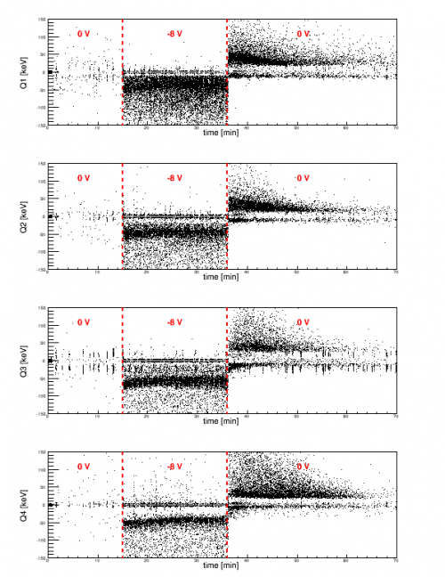Signal vs. time while changing the DCRC bias. Left: Positive 8 V bias, Right: negative 8 V bias When grounded after biasing, some signal of opposite plarity is seen to persist, indicating the presence of an accumulated counter-bias in the detector. At positive bias, channels 2 and 3 have 2 distinct gains between minutes 20 and 30.

Figure 12
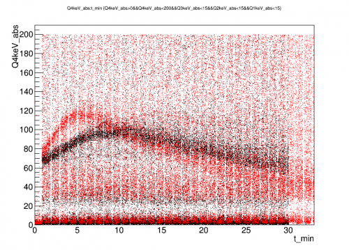Effect of increasing the overall rate with an external 133Ba source. All data was taken at 6V. The red points were taken with the Ba source near the fridge. The initial slope increases by a factor of ~2.2 while the energy deposition rate is only ~15% higher.

Figure 13
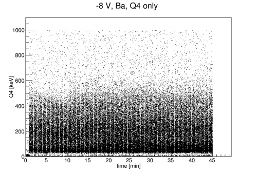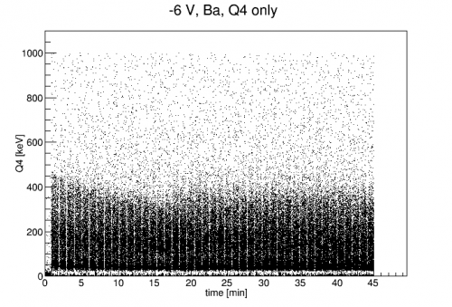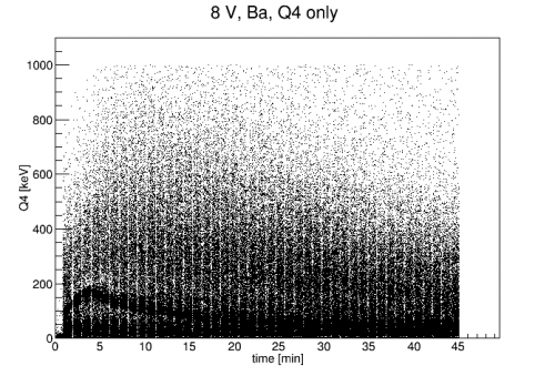
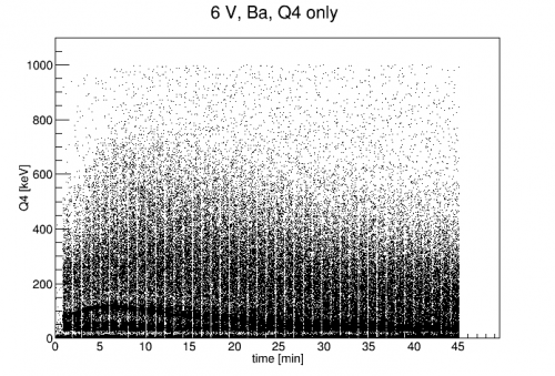
The high energy background spectrum is seen to roughly follow the 60 keV line behavior. At positive biases, it has a strong peak at the beginning of the run, then settles. At negative biases, it has a small decrease at the beginning. This indicates that whatever is causing this behavior is 1) Not just local to the sources and 2) depends on bias polarity of all events.

Figure 14
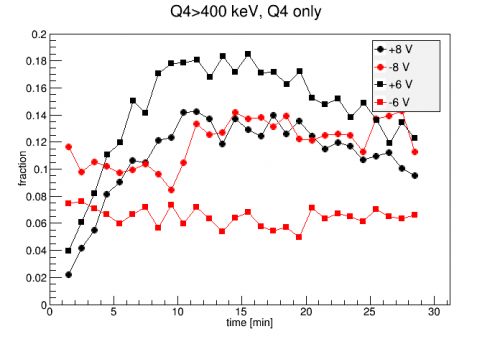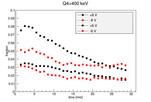The fraction of events in each minute which are above 400 keV in Q4. Includes cut for Q4-only events.	Same as on the left, but no cut for Q4-only events.

The left plot of Fig. 14 shows the fraction of events above 400 keV in each minute of Ba data. It indicates that whole energy spectrum has a time-dependent amplification similar to the 60keV line. The positive biases seem to peak at 10-15 minutes, though the 60keV line does so at ~5 min. The negative biases are roughly flat. Note that the shape of these curves depends not just on the amplification factor but on the spectrum as well. However, this does not much change the flat behavior nor does it change where the positive bias data maximizes.

Figure 15
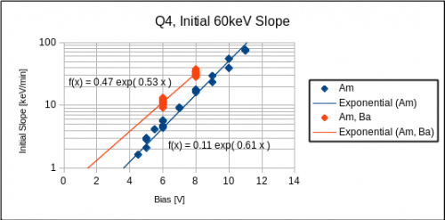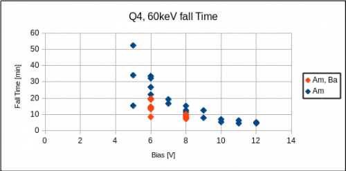Measured initial slopes and exponential fall times as a function of bias voltage. The initial slopes closely follow an exponential of bias voltage. The fall times may also be exponentially decreasing with increasing bias. However, the uncertainty in fall times is significant at low bias. When the peak is only slowly and weakly falling, it is difficult to get a plausible fit. This is seen by the scatter in measured points at low bias.