What is the current best PSD estimate from series 07221203_2025?
WARNING (22 October 2026): the sample time has
changed. The phonon sample period is 0.8 µs (1.25 MHz),
not 1.6 µs (625 kHz); a 4096-sample trace is 3.2768 ms. This
note, its figures and its HDF5 file were made with 1.6 µs until
2026-10-22, which was wrong (see The sample period in
python/README.md). What changed in this note:
- The frequency axis of Figures 4 and 6 now reaches 625 kHz (it ended at 312 kHz); every frequency is twice what it was, so a feature the old figures showed at 100 kHz is at 200 kHz. The frequency bins are 306 Hz apart (153 Hz before), from 306 Hz to 625 kHz.
- The PSD is divided by 2 and the amplitude spectral density by (the factor in the definition), so the ASD values quoted for Figure 4 changed: the plateau above 100 kHz is 1.70e-3 to 1.74e-3 counts/√Hz in the three DCRC1 channels (it was 2.37e-3 to 2.59e-3 in five channels), and between 1 and 10 kHz the six sensors are at 6.29e-3 to 1.10e-2 counts/√Hz (6.71e-3 to 1.23e-2 for the six, with the input now known to be the NaI trigger at 2.61e-3, before). The channel names in this line are those of the channel-map box below. Because the bands 1 to 10, 10 to 100 and above 100 kHz stay the same while the frequencies doubled, they now cover different parts of the spectrum.
-
in the PSD definition is 0.8 µs, the code block no longer sets
sample_period_s(the library default is used), and the HDF5 filepsd-clean-randoms-07221203_2025_F0001.h5hassample_period_s= 8e-07 and the frequencies of the new axis, so any analysis that used its frequencies must be redone. - Unchanged by the sample time: everything counted in samples or counts (the cuts, the 101 and 141 events (the strictest cut’s 31 is now 34, see the next box), the traces and pulse heights in all the figures other than 4 and 6 (they are identical pixel for pixel), the sample numbers quoted for the events).
- The Code repository section is pinned to the commit of the latest
re-run (
18c4babfor the notebooks, figures and file,ade25dffor the library).
WARNING (22 October 2026): the channel map has
changed. The table columns used for the channel names were the
wrong ones for this series. It is read out on Side 2,
so one uses the Label and HV output, Side 2 readout
columns of the Run 76 Setup table: there are six sensors, all on
Side 2, on DCRC1 and DCRC3; DCRC4 pA is the input of
the NaI trigger signal and the other five inputs are not
connected (python/pulse_channels.py, since 2026-10-22).
What changed in this note:
- The channel names. The dump channel (0, 3) was
Side1pFand isSide2pE(PES2); (1, 0) wasSide1pEand isSide2pB(PBS2); (1, 1) wasSide1pBand isSide2pA(PAS2); (1, 3) wasSide2pEand isSide2pD(PDS2); (2, 0) wasSide2pB(PBS2) and is the NaI trigger input.Side2pC(PCS2, 0 / 0) andSide2pF(PFS2, 0 / 1) are as before. Everything keyed by (detector, channel), the cuts, the event numbers and counts, is unchanged. - No Side 1. Figure 1 shows one face with six regions instead of two faces with seven working channels (it is now a generic layout, the counts of randoms are in the table above it; Appendix C, new, draws both faces); the colours of the other figures are by board (blue DCRC3, orange DCRC1), and the by-side figures (4, 6) are by board; Figures 3 and 8, and the text about the cut “on one channel of each side”, are now about one channel on each board.
- The cut we use is made on PAS2 (the old PBS1), a channel of DCRC3. Its 101 events are the same.
- PBS2 is gone as a phonon channel. The caveat about it (flat, low spectrum, maybe superconducting) is replaced: DCRC4 pA is the NaI trigger input.
- Numbers that changed. The strictest cut (every
working channel) keeps 34 randoms, it was 31: three
randoms failed only in the NaI input, which is no longer one of the
channels. The amplitude of each sensor is the same as before under its
new name; the 101-to-34 comparison and the lists of channels changed
with the names. In the HDF5 file, the six channel groups are
Side2pAtoSide2pF(the oldSide1pBgroup isSide2pA), withside= 2 and the new attributesboard_inputandhv_output; the NaI input has no group. - Not settled. The A/B order on DCRC1 is the table’s
(A is
Side2pC, B isSide2pF); the explanatory text next to the table writes it the other way round, which we take to be a typo (the Trello page of the notebook carries a marked copy). The board order and the Side-2 readout of the December series are inferred (Data and setup).
Code repository
All code is pinned to two commits: buddy’s notebooks, the saved HDF5
file and the figures to 18c4bab, the commit of the re-run
with the corrected sample period (0.8 µs) and the channel map of the
Side-2 readout, and the library in python/ to
ade25df. Each link shows the file as it was when the
results below were made, which may be older than the latest version, and
the file may have moved since (see
data_analysis/README.md). On the published page a small
“latest” link after each one opens the file on develop
today.
psd-clean-randoms-buddy.ipynb: the spectra of every channel from theclean_randomscut, and the saved HDF5 filepsd-clean-randoms-07221203_2025_F0001.h5(Noise Power Spectral Densities).chan0-cut-on-all-channels-buddy.ipynb: how good the PCS2 cut (the channel names are explained under Data and setup) is on the other channels, and the definition of the cut we use (clean_randoms) (Selection of Randoms in All Channels, Data and setup for the timing of the randoms, Appendices A and B).detector-faces-buddy.ipynb: the drawing of both faces of the detector (Appendix C).noise-psd-randoms-buddy.ipynb: the channel map and the noise spectra of the 34 events of the strictest cut (Data and setup, Appendix A).extract_odb_facts.pyandodb-facts-07220916_2200.json: the run configuration of series07220916_2200(board order, QET biases, random rates) read from its raw file, which is not in the repository, and the numbers it gave; section 12 ofnoise-psd-randoms-buddy.ipynbprints them (Data and setup, Caveats).pulse_channels.py,pulse_cuts.pyandpulse_quantities.py: the library for the channel names, the randoms and excursion-band cuts, and the PSD.
Data and setup
We are using the file 07221203_2025_F0001, which is series
07221203_2025, Dump 1. The first 1000 events are “random” triggers (the
“Beginning of Run Randoms,” BORR, taken at about 20 Hz: 1000 events in
49 seconds); random triggers are snapshots of our detector traces taken
at any time (rather than when a pulse occurs) to sample the noise
environment. The line in the third code block of the noise-psd-randoms-buddy.ipynb
notebook shows the randoms cut defined as
quiet_noise = pc.excursion_band(pulses, config_500) & (np.log10(bstd_500) < 0.5)
in addition to selecting the trigger specification for random events.
The other 8 of the 1008 events that carry the randoms label are “in-run”
randoms: they are spread through the rest of the dump, one every 1 to 2
seconds (all 8 in the last 9 seconds of the dump; the timestamps have
one-second resolution). The run configuration of series
07220916_2200 lists 5 Hz for in-run randoms, which does not
match what we see here, so that rate should not be assumed for this
series.
Note. The trigger-type labels in the dump’s
.csv are the wrong way round. The column
trigger_type has two values, Physics and
Unknown. By their names one would read Physics
as an event triggered by a pulse and Unknown as a trigger
of undetermined type. In this dump it is the opposite: the first 1000
events, which are the Beginning of Run Randoms (the run configuration
asks for 1000 randoms at 20 Hz, and these 1000 events span 49 s, which
is 20.4 Hz), are all labelled Physics, and the other
events, 509 in this dump, are labelled Unknown. So we take
Physics to mean a random trigger and Unknown
to mean a real (pulse) trigger, which is what pc.randoms
and pc.real_triggers do. This is a working assumption:
nothing in the data files or the DAQ documentation we have confirms it,
and the two functions are tagged under development for that reason (see
Note
2a).
It may also be useful to have a diagram of the detector and which channels are working during the R76 run period at UMN. The figure below was reconstructed from the archive of the UMN Wiki.
How we found which channel is which. The data are numbered by detector (0 to 2) and channel (0 to 3), but there is one detector, S104, read out by three four-channel electronics boards (DCRC1, DCRC3, DCRC4). We matched them to the detector’s channels in four steps:
- The channel table and the readout. The
Setup table of the UMN
Run 76 summary lists the 12 sensors of the detector with a Label
(
Side1pAtoSide2pF) and, for a Side-1 readout and for a Side-2 readout, the HV connector pin each is wired to. Matt Fritts’s explanation of the table (page 28 of the notebook N-MISC-23-001) says to use the Label and HV output, Side2-readout columns: HV1 and HV2 are the two D-subs the DCRCs plug into, and the header of a run-diary page from late in the run, when the detector was left in Side-2 readout, says that HV1 has DCRC3, HV2 has DCRC1 and the NaI trigger signal goes to DCRC4. The December 2022 series is after that change, so it is a Side-2 readout. (An earlier version of this note used the table’s DCRC (2-sided) column and found twelve channels on two sides, which was wrong for this readout.) - The pins. In Side-2 readout HV2 pA, pB, pD are
Side2pC,Side2pF,Side2pE(DCRC1) and HV1 pA, pB, pD areSide2pB,Side2pA,Side2pD(DCRC3); pC is not used. Matt’s text next to the table writes the DCRC1 order as pF, pC, pE; the table and the 2022 diaries (“DCRC1pA = Side2pC”) agree with each other, so we take the text to be a typo. This is not confirmed with Matt. - The board order. The table does not say which board
is detector 0, 1 or 2. The raw file of another Run 76 series
(
07220916_2200; the raw file for series07221203_2025, the one analysed here, is not on NSDF) holds the run configuration. It enables boards DCRC1, DCRC3 and DCRC4, and the three records of each event carry the codes 9, 11 and 12, which are the board numbers plus 8. So detector 0, 1, 2 = DCRC1, DCRC3, DCRC4. This is inferred and not confirmed. - The channels within a board. We assumed the dump’s channels 0 to 3 are the board inputs pA to pD in order. The data agree: the inputs whose signal never changes (channel 2 of DCRC1 and DCRC3, the pC inputs that Side-2 readout does not connect, and channels 1 to 3 of DCRC4) are the ones that configuration lists with zero QET bias, and DCRC4 channel 0, with its feedback disabled, is the NaI trigger input.
The mapping is kept in python/pulse_channels.py,
marked as under development, and section 7 of that notebook, noise-psd-randoms-buddy.ipynb,
gives the evidence.
Channel names. In the text a channel is written as
P, the letter of its sensor, and its side: PCS2 is the phonon channel C
on Side 2. The library, the tile titles of the figures and the HDF5 file
of the PSDs use the form Side2pC for the same channel, and
the dump numbers it as detector 0, channel 0. The six sensors, all on
Side 2:
| In the text | Library and figures | Dump (detector / channel) | Board and input | Randoms that pass its own quiet-noise cut |
|---|---|---|---|---|
| PCS2 | Side2pC |
0 / 0 | DCRC1 pA | 141 |
| PFS2 | Side2pF |
0 / 1 | DCRC1 pB | 107 |
| PES2 | Side2pE |
0 / 3 | DCRC1 pD | 109 |
| PBS2 | Side2pB |
1 / 0 | DCRC3 pA | 161 |
| PAS2 | Side2pA |
1 / 1 | DCRC3 pB | 101 |
| PDS2 | Side2pD |
1 / 3 | DCRC3 pD | 180 |
The other six inputs are not sensors: DCRC4 pA (dump 2 / 0) is the input of the trigger signal of the NaI array, and DCRC1 pC, DCRC3 pC, DCRC4 pB, pC and pD are not connected (their signal never changes).
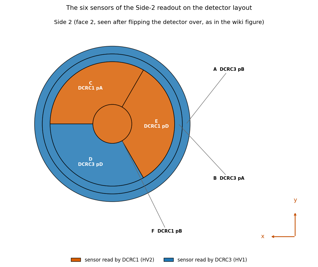
Figure 1: The six sensors of detector S104 on Side 2, the face that is read out in this series (as seen after flipping the detector over). Each region is coloured by its readout board, DCRC1 (orange) or DCRC3 (blue), and labelled with its letter, its board and input (the number of randoms that pass each sensor’s own quiet-noise cut is in the table above). The other six inputs are not on the detector. Appendix C draws the whole detector, with the face that is not read out.
The question
Based on this series’ Beginning of Run Randoms (BORR), what is our best estimate for the noise environment of the experimental setup? The noise environment is typically summarized in terms of the Power Spectral Density (PSD).
Selection of Randoms in All Channels
Typically, BORR are taken in the first events of the first “dump” (file) of a series’ raw data. In this series that is the case and there are 1000 BORR. Often some of the initial traces are “contaminated” with a real physics pulse that just happened to be in the random’s readout window. We call this a “pileup” pulse. Those occurances can mess up the noise computation and therefore the extracted pulse amplitudes; pulse amplitudes are used to estimate the energy deposited in each event. Here I describe how we make a cut on the data to be sure those pileups are removed.
This sort of thing has been done on one channel, PCS2, and it is the
topic of Note
2 and Note
2a. Note 2 develops the noise-pulse selection: an excursion cut on a
500-sample pretrigger window (the Tight band) together with a cut on the
baseline scatter, log10(bstd) < 0.5, which keeps 179 of
the 1517 traces. Note 2a adds the trigger cut that keeps only the
randoms, 141 of those 179 (the other 38 are real triggers), and looks at
how the baseline scatter changes with time.
To use that cut I have to decide how to apply it to all of the channels. A pileup should show up in all channels simultaneously, because the origin is a real physics event. It is possible the amplitude in some channels could be small enough so that it’s not obvious. Figure 2 is a plot based on the cut for PCS2 only (see the Data and setup section). To my slight surprise I found that this cut does not remove some traces that are either glitches or tails of pulses in the DCRC3 channels. I don’t want those pulses in the noise sample.
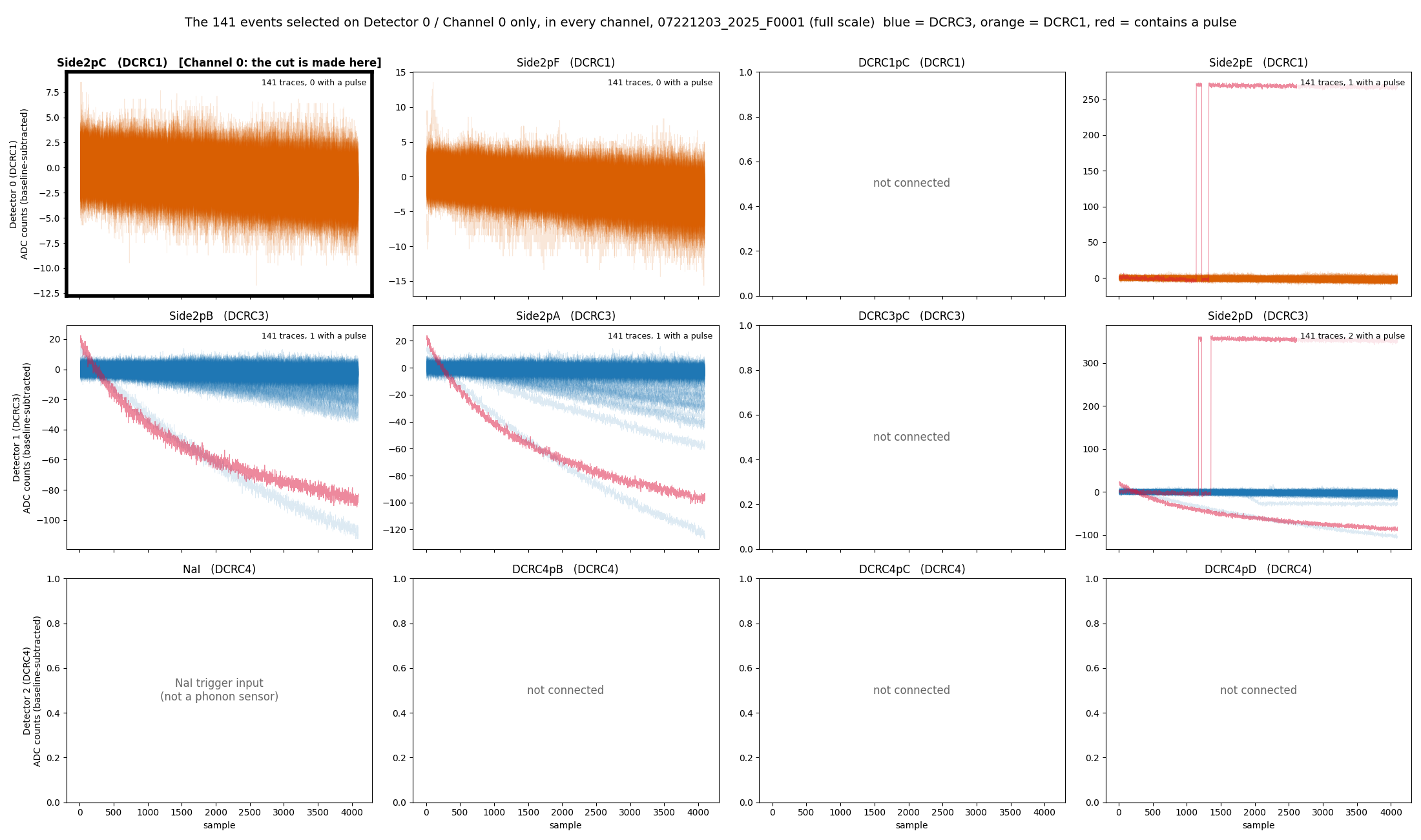
Figure 2: The 141 randoms that pass the PCS2 cut, in every channel. One tile per channel (rows are the boards DCRC1, DCRC3 and DCRC4); the traces are drawn over each other with transparency, baseline-subtracted, on a free vertical scale. The cut is made on PCS2 (framed). Blue is DCRC3, orange is DCRC1, and red marks a trace that contains a pulse. The 6 tiles with grey text are the inputs that are not sensors. Several traces carry large baseline ramps in the DCRC3 channels even though they are quiet in PCS2.
Based on what was seen in Figure 2. I developed a cut that will select noise for PAS2. It will hopefully not be as strict as requiring the analogous cut to be true on all channels. That leaves only 34 traces (see Appendix A).
Instead of doing all channels I selected instead one channel on each board to apply the standard cut to and then took the logical “AND.” In that case the remaining number of traces was somewhat small (71) but the quality looked pristine.
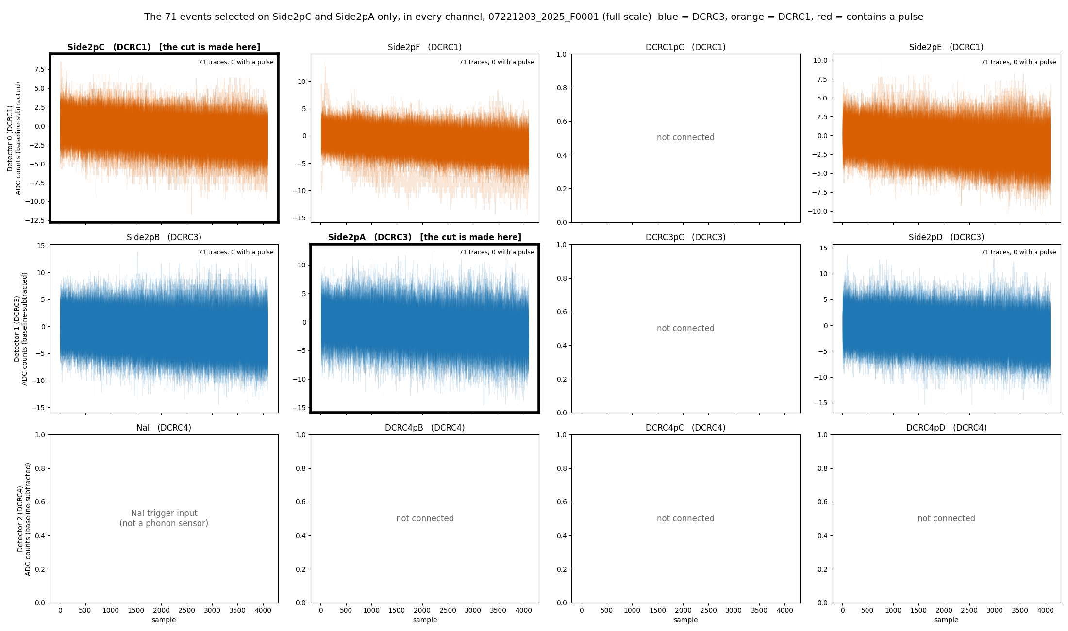
Figure 3: The randoms that pass the cut on one channel of each board, in every channel. The cut is the quiet-noise cut on PCS2 (DCRC1) and on PAS2 (DCRC3), both framed. One tile per channel, with the traces drawn over each other with transparency on a free vertical scale. Blue is DCRC3, orange is DCRC1, and red would mark a trace that contains a pulse. The 6 tiles with grey text are the inputs that are not sensors.
While setting this up in the Jupyter notebook chan0-cut-on-all-channels-buddy.ipynb,
I checked if there were similar traces left in the DCRC1 channels after
selecting on PAS2 (DCRC3), just like we saw in the DCRC3 channels after
selecting on PCS2 (DCRC1). Appendix B
shows the traces left in the DCRC3 channels after the PCS2 cut (Figure
7), and then the PAS2 cut itself (Figure 8). To my surprise there
were not traces in the DCRC1 channels that were very apparent.
That means that for some reason cutting on PAS2 is more pure than
cutting on PCS2. Since cutting on PAS2 alone is also less restrictive
than the combined cut by definition, this led to more accepted randoms
(101, compared with 71 for one channel on each board and 34 for all
channels).
We will use this cut going forward: the cut of Notes
2 and 2a (a random trigger in the Tight excursion band with
log10(bstd) < 0.5) made on PAS2 (DCRC3). In the notebook
it is defined in one place, clean_randoms_cut, and the
selection it makes is called clean_randoms.
Noise Power Spectral Densities
The key parameter we want to get out of pulses in these detectors is the overall “amplitude” because it should be proportional to the energy deposited in a scattering event. That’s hard to do for the small signals (near the noise baseline) that we have for dark matter direct detection (the expected recoil spectrum rises roughly exponentially toward low energy, with no turnover; Lewin and Smith [1]) so we use an algorithm called the Optimal Filter (OF) (Gatti and Manfredi [2]; Golwala [3]; Press et al. [4]; Szymkowiak et al. [5]) instead of a simpler procedure like integrating the pulses. The crucial part of the OF is that it takes into account the electronic noise environment of the sensor, rather than blindly integrating. The noise is summarized by the Power Spectral Density (PSD) constructed with traces that have no pulses present–the ones we are selecting here.
The PSD is sort of like the standard deviation of different frequency components in a trace (any trace can be written as a sum of sinusoids of different frequencies, the Fourier decomposition [4]). The PSD can be calculated for discrete data sampling as below, by averaging the squared Fourier amplitudes of many traces (Welch [6]):
Take a trace of
samples
,
,
taken every
(here
),
with its baseline subtracted. Its discrete Fourier transform is
,
with
(
is even here), which are the non-negative frequencies, all that the
one-sided PSD needs. Bin
sits at the frequency
,
from zero
()
up to the Nyquist frequency
().
Averaging over
traces with no pulse in them (here the
traces of the clean_randoms cut, or the 34 of Appendix A),
the one-sided PSD is
where
is trace
and
its transform. The amplitude spectral density is
,
in
counts/.
The factor 2 folds the negative frequencies onto the positive ones (it
is left out for the zero-frequency and Nyquist bins), and the
and
make
independent of the trace length and the sampling rate, so that its
integral over frequency equals the mean square of the trace (its
variance, if the trace has zero mean). Here
= 4086, the length of a trace after the leading glitch samples are
dropped, so there are 2044 bins, from 306 Hz (the first non-zero bin) to
625 kHz; the zero-frequency bin is not plotted. This is the convention
used in the notebook (noise-psd-randoms-buddy.ipynb);
Note 3 plotted the raw
instead, which differs from
only by the constant
.
Conventions. We use one-sided spectra: the PSD above, in counts²/Hz, and the amplitude spectral density (ASD) , in counts/, which is the quantity the figures show and the usual way to quote noise. Golwala [3] (appendix B, pp. 409 to 418) uses a different convention in three ways. His Fourier transform has the factor on the forward transform (p. 412), so his is our . His PSD is two-sided, with equal to the variance (p. 415). He estimates it as , averaged over noise traces, with (p. 417); the averaging over traces is the same as ours. In our terms for , so his amplitude is our ASD divided by . He also notes that the quantity usually quoted, , is often wrongly called the PSD (p. 415). The difference matters when the spectrum goes into the optimal filter, whose expected resolution is for a pulse template (his equation B.1, p. 418). Written with our one-sided it is , and using in his formula unchanged would be off by a factor of 2. The template must use his scaling of the Fourier transform too.
Figure 4 shows the amplitude spectral density of the 101 events of
the clean_randoms cut, the cut used from now on. Above 100
kHz it is flat, between 1.70e-3 and 1.74e-3 counts/√Hz in the three
DCRC1 channels PCS2, PFS2 and PES2; the narrow lines of the DCRC3
channels raise their means to 1.98e-3 (PAS2), 2.64e-3 (PBS2) and 2.93e-3
(PDS2) counts/√Hz. Between 1 and 10 kHz the amplitude is 6.29e-3 to
1.10e-2 counts/√Hz in the six channels.
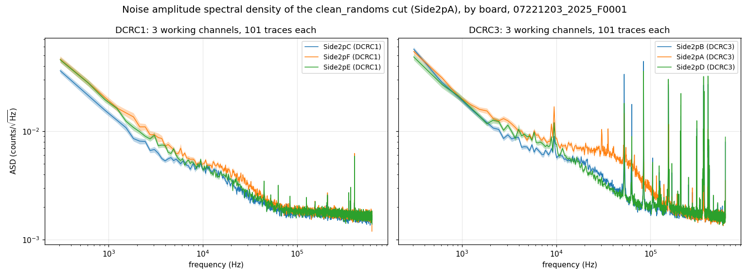
Figure 4: The noise amplitude spectral density of the 101
randoms of the clean_randoms cut, by board. DCRC1
on the left (3 sensors) and DCRC3 on the right (3 sensors), one colour
per channel within each panel (the colours are not shared between the
panels). Each curve is the one-sided amplitude spectral density
(counts/√Hz), the square root of the mean PSD over the 101 events as
defined above, and the thin band around it is the uncertainty on the
mean (one standard error carried to the square root, 0.049 to 0.050 of
the value in every channel). Both panels share the same axes. The inputs
that are not sensors are not shown.
References
- J. D. Lewin and P. F. Smith, “Review of mathematics, numerical factors, and corrections for dark matter experiments based on elastic nuclear recoil,” Astroparticle Physics 6(1), 87 (1996), doi:10.1016/S0927-6505(96)00047-3.
- E. Gatti and P. F. Manfredi, “Processing the signals from solid-state detectors in elementary-particle physics,” Rivista del Nuovo Cimento 9(1), 1 (1986).
- S. R. Golwala, Exclusion Limits on the WIMP-Nucleon Elastic-Scattering Cross-Section from the Cryogenic Dark Matter Search, PhD thesis, University of California, Berkeley (2000), Appendix B, “Noise and Optimal Filtering”.
- W. H. Press, S. A. Teukolsky, W. T. Vetterling and B. P. Flannery, Numerical Recipes in C: The Art of Scientific Computing, 2nd ed. (Cambridge University Press, 1992): chapter 12, Fast Fourier Transform, p. 496; chapter 13, section 13.3, Optimal (Wiener) Filtering with the FFT, p. 547.
- A. E. Szymkowiak, R. L. Kelley, S. H. Moseley and C. K. Stahle, “Signal processing for microcalorimeters,” Journal of Low Temperature Physics 93(3-4), 281 (1993).
- P. D. Welch, “The use of fast Fourier transform for the estimation of power spectra: a method based on time averaging over short, modified periodograms,” IEEE Transactions on Audio and Electroacoustics 15(2), 70 (1967), doi:10.1109/TAU.1967.1161901.
Caveats
- DCRC4 pA is not a phonon channel. An earlier
version of this note listed it as PBS2, a seventh working channel with a
flat spectrum well below the others, and wondered whether it was
superconducting. With the corrected channel map it is the input of the
trigger signal of the NaI array (DCRC4 pA, baseline about 7950 counts),
so it has no phonon spectrum; the run configuration we read for another
series (
07220916_2200) lists zero QET bias on all four DCRC4 channels and the feedback of channel 0 disabled, which fits an input that is not a sensor. The UMN wiki mentions the NaI trigger signal in DCRC4 pA in its diaries; the page of the run summary shows an example of it. - The A/B order of DCRC1 is the table’s. The Setup
table has HV2 pA on
Side2pCand HV2 pB onSide2pF; Matt Fritts’s text next to the table writes A, B, D as pF, pC, pE. We take the text to be a typo, because the table and the 2022 diaries agree. If the text were right, the names PCS2 and PFS2 would swap. Not yet confirmed with Matt. - The Side-2 readout of this series and the board order are inferred. The Side-2 readout comes from the header of run-diary pages from late in the run, not from the pages of December 2022, and the order DCRC1, DCRC3, DCRC4 of detectors 0, 1, 2 from the run configuration of another series (Data and setup).
Results
The cut: clean_randoms
The selection of randoms that we use from now on is called
clean_randoms. It is the cut of Notes 2
and 2a, made on PAS2 (DCRC3): a random trigger (pc.randoms)
whose trace falls in the Tight excursion band of the 500-sample
pretrigger window (pc.excursion_band) and has
log10(bstd) < 0.5. In series 07221203_2025,
dump F0001 it keeps 101 of the 1008 randoms, none with
a pulse or a big tail in any channel (Appendix B). It is defined by the
function clean_randoms_cut in chan0-cut-on-all-channels-buddy.ipynb
(section 13), and the code below is that function.
clean_randoms is a True/False value for every event of the
dump; because the three boards share their events in the same order, the
same list selects the clean random traces of every channel.
import sys
from pathlib import Path
import numpy as np
from nsdf_dark_matter.idx import load_all_data

REPO = next(p for p in [Path.cwd().resolve(), *Path.cwd().resolve().parents] if (p / "python" / "pulse_io.py").exists())
sys.path.insert(0, str(REPO / "python"))
import pulse_io as pio
import pulse_quantities as pq
import pulse_cuts as pc
from pulse_config import PulseConfig

config = PulseConfig(pretrigger_samples=500, glitch_samples=10)     # the sample period is the library default, 0.8 us

def clean_randoms_cut(pulses, trigger_types, config=config):
    """Randoms with no pulse: a random trigger in the Tight excursion band with log10(bstd) < 0.5."""
    with np.errstate(all="ignore"):
        quiet = pc.excursion_band(pulses, config) & (np.log10(pq.bstd(pulses, config)) < 0.5)
    return pc.randoms(trigger_types) & quiet

cdms = load_all_data(str(Path.home() / "idx" / "07221203_2025_F0001"))
det1 = pio.filter_by_detector(cdms.get_detector_ids(), 1)
_, pulses = pio.load_channel_batch(cdms, det1, 1)               # Side2pA: detector 1, channel 1
clean_randoms = clean_randoms_cut(pulses, pio.trigger_types(cdms, det1))   # True for the events of the cut
print(clean_randoms.sum(), "of", len(clean_randoms), "events")

det0 = pio.filter_by_detector(cdms.get_detector_ids(), 0)
_, other = pio.load_channel_batch(cdms, det0, 0)                # any other channel: same events, same order
traces = other[clean_randoms]                                   # its clean random traces
print(traces.shape)
Run it from inside the NSDF-Data folder, after
downloading the dump to ~/idx. It prints
101 of 1517 events and (101, 4096). The
library prints a warning that pc.randoms is under
development, because it assumes the trigger labels are swapped (Note
2a).
The PSDs
I’ve made the current best estimate of the noise spectrum
specifically focusing on the series 07221203_2025. The
spectra are accessible via psd-clean-randoms-07221203_2025_F0001.h5
file (pinned to 18c4bab, 435 kB), and can be accessed
by:
import h5py
import numpy as np

with h5py.File("data_analysis/R76/student/buddy/psd-clean-randoms-07221203_2025_F0001.h5", "r") as f:
    freq = f["frequency_hz"][:]                       # Hz, shared by all channels
    events = f["event_numbers"][:]                    # the 101 clean_randoms events
    asd = {name: (g["asd_mean"][:], g["asd_sem"][:])  # counts/sqrt(Hz), one-sided, and its standard error
           for name, g in f["channels"].items()}

mean, sem = asd["Side2pA"]
print(len(events), "events;", len(asd), "channels:", ", ".join(asd))
print(f"Side2pA at {freq[100]:.0f} Hz: {mean[100]:.2e} +/- {sem[100]:.1e} counts/sqrt(Hz)")
Run it from the NSDF-Data folder. It prints the number
of events and the 6 sensors (Side2pA, Side2pB,
Side2pC, Side2pD, Side2pE,
Side2pF: PAS2, PBS2, PCS2, PDS2, PES2 and PFS2 in the
notation above); the inputs that are not sensors have no spectrum. Each
channel group has the attributes detector,
channel, side (2), dcrc,
board_input and hv_output. For each channel
the file holds the amplitude spectral density of the 101 events of the
clean_randoms cut (asd_mean, one-sided, in
counts/√Hz) and its standard error (asd_sem), and the PSD
it is the square root of (psd_mean and
psd_sem, in counts²/Hz); the layout of the file is
described in section 7 of psd-clean-randoms-buddy.ipynb,
which also makes them. The caveats above apply.
Next steps
Next steps. There are two possibilities:
- Calibrate the PSD in amps. Get the calibration for the PSD so that we can write the noise in amps, and later compare it with the theoretical best resolution. This will probably be difficult, because it is not clear that the UMN wiki has the necessary information. As far as we found, the DCRC v3 page gives the size of one ADC bin (14 bits over ±1.25 V, 152.6 µV per bin) but not the feedback resistor, the SQUID coil ratio or the TES bias power, which are needed to turn counts into amps.
- Find triggered pulses. Find triggered pulses in dump 2 or later, so we can continue on the path of running the Optimal Filter on pulses.
Appendix A: the strictest cut (every working channel)
The strictest version of the selection keeps a random only if it
passes the quiet-noise cut (the Tight excursion band and
log10(bstd) < 0.5) in every working
channel. Six of the 12 inputs are sensors and work, and the
other six (the NaI trigger input and five unconnected inputs) are left
out, so the cut is applied to the six. It keeps 34 of the 1008
randoms (31 in the earlier version, which counted the NaI input
as a seventh channel: three randoms failed only there), far fewer than
the 141 that pass on PCS2 alone. Each of the six sensors passes the cut
for only 101 to 180 randoms on its own, and the events that fail are not
the same in all of them. Any two of those channels share 62% to 89% of
the smaller set (well above the 11 to 29 events expected by chance), but
each further channel removes more, so only 34 events pass in all of
them, 34% of the 101 of PAS2, the strictest channel. The Tight excursion
band does most of the rejecting: only 116 to 189 of the 1008 randoms
fall in the band on each of the six channels, while the
log10(bstd) < 0.5 condition keeps 770 to 895.
Figure 5 shows the 34 traces themselves in every channel (section 12
of chan0-cut-on-all-channels-buddy.ipynb):
none of them has a pulse or a ramp, and they all look like noise, but
there are only 34 of them. Figure 6 shows their noise amplitude spectral
density, the mean of the 34 traces in each channel (section 11 of noise-psd-randoms-buddy.ipynb).
With so few traces the spectra are jagged from bin to bin, and no spread
between the traces is drawn. This is why a cut that is not required to
hold on all channels, and so keeps more traces, is worth looking
for.
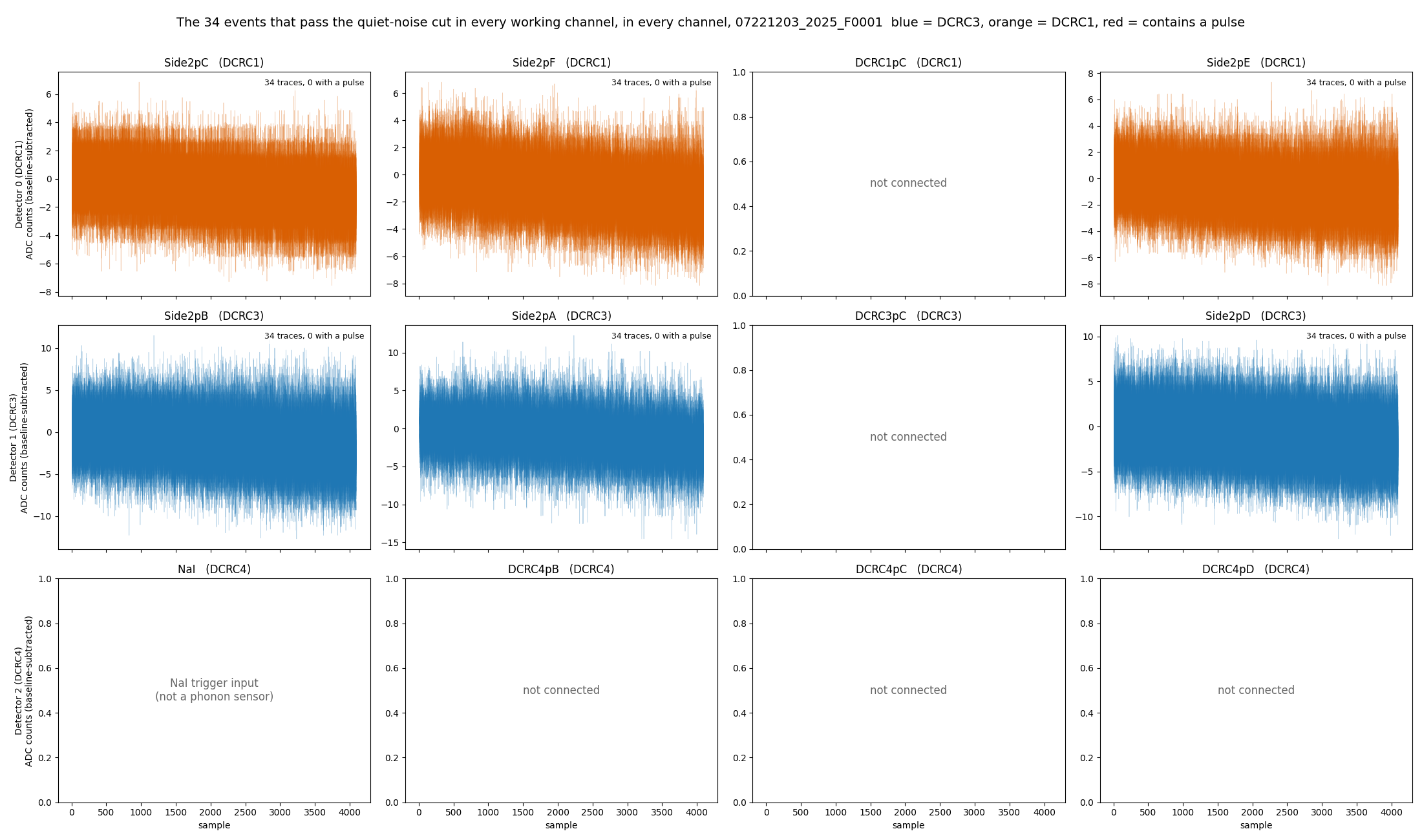
Figure 5: The 34 randoms that pass the quiet-noise cut in every working channel, in every channel. One tile per channel (rows are the boards DCRC1, DCRC3 and DCRC4), with the traces drawn over each other with transparency, baseline-subtracted, on a free vertical scale. Blue is DCRC3 and orange is DCRC1; no trace contains a pulse. The 6 tiles with grey text are the inputs that are not sensors.
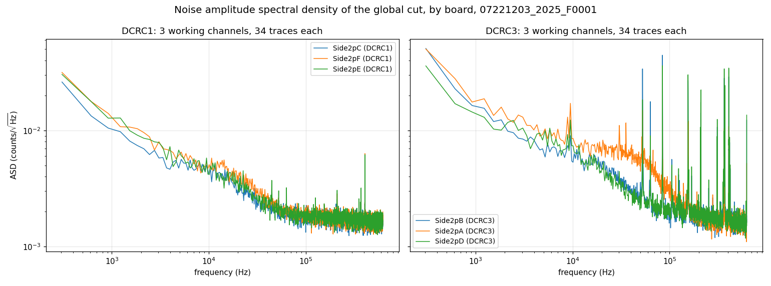
Figure 6: Noise amplitude spectral density of the 34 randoms that pass the quiet-noise cut in every working channel, by board. DCRC1 on the left (3 sensors) and DCRC3 on the right (3 sensors), one colour per channel within each panel (the colours are not shared between the panels). Each curve is the one-sided amplitude spectral density (counts/√Hz), the square root of the PSD computed as the mean over the 34 traces of the squared Fourier amplitude of each trace (baseline-subtracted, first samples skipped) scaled to a one-sided density; the spread between traces is not drawn. Both panels share the same axes. The inputs that are not sensors are not shown.
Appendix B: the cut on PCS2 and the cut on PAS2
What the PCS2 cut lets through. Of the 141 randoms that pass the cut on PCS2, 10 have a pulse or a big tail in some channel: 2 contain a pulse and 8 more have a baseline sag of more than 30 counts across the trace. Figure 7 shows only these 10, each in its own colour, which is the same in every tile. Event 10550 (light green) steps up by about 273 counts in PES2 (at sample 1139) and by about 359 counts in PDS2 (at sample 1171), falls back at sample 1219 in both, and steps up again at samples 1323 and 1355. Event 10034 (light blue) is a long decay in the three DCRC3 channels, down to about -100 counts. The big tails are in DCRC3, and the sag is largest in PAS2 for 8 of the 10 events (up to 133 counts for event 10027). In the framed PCS2 tile the same 10 traces lie in the same noise band as all the others, which is why the PCS2 cut cannot see them.
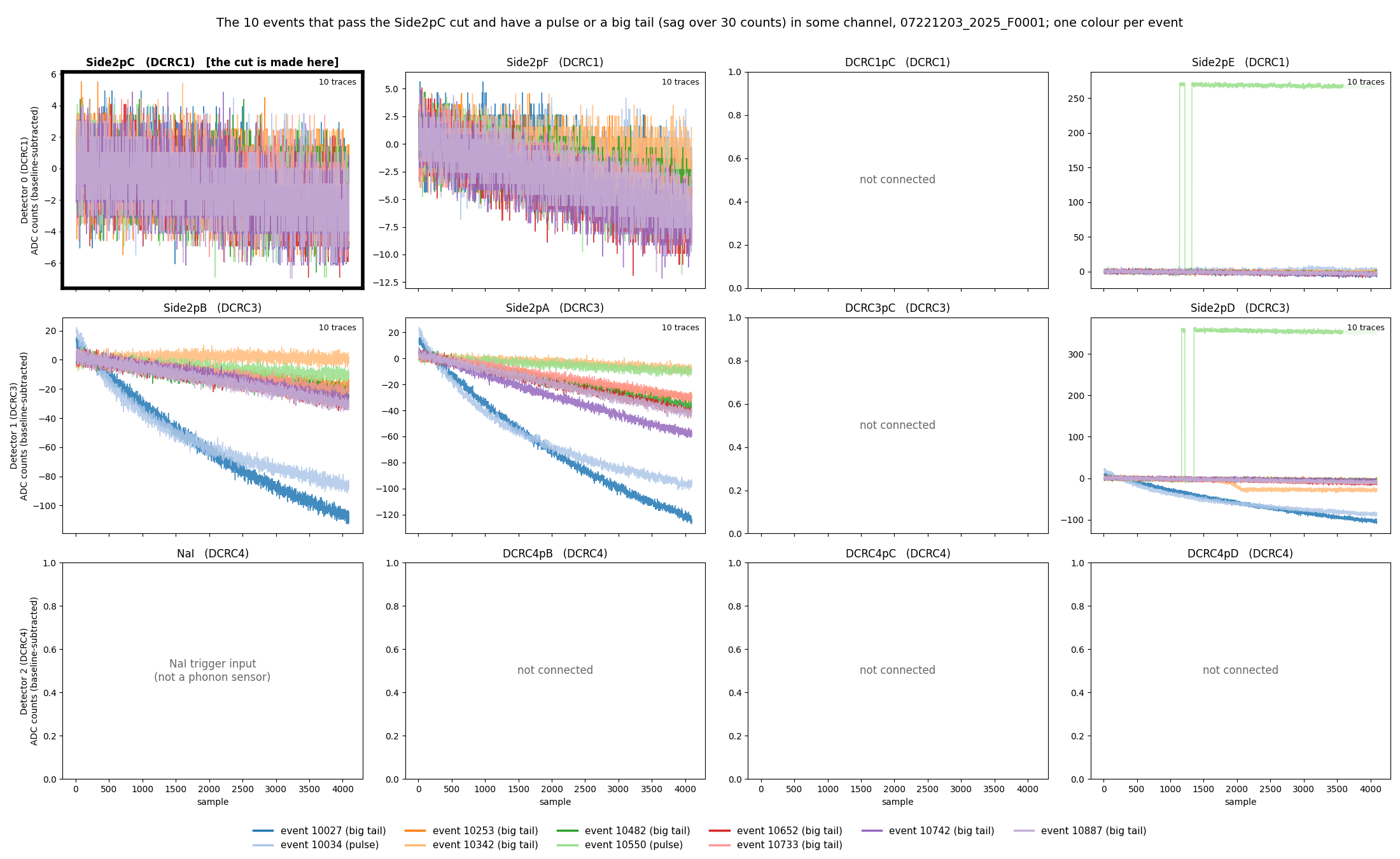
Figure 7: The 10 randoms that pass the PCS2 cut but have a pulse or a big tail in some channel. They are drawn in every channel, but the tails are in a few of them (mainly the three DCRC3 channels); the other channels show only noise. The cut is made on PCS2 (framed). One colour per event, the same in every tile, and the legend gives the event numbers and whether each has a pulse or a big tail (a sag of more than 30 counts across the trace). One tile per channel (rows are the boards DCRC1, DCRC3 and DCRC4), baseline-subtracted, on a free vertical scale. The 6 tiles with grey text are the inputs that are not sensors.
The cut on PAS2 only. The cut we will use is the one
of Notes 2 and 2a on PAS2 alone: a random whose trace passes the Tight
excursion band and log10(bstd) < 0.5 on that channel. It
keeps 101 of the 1008 randoms, more than the 71 of the
cut on one channel of each board and the 34 of the cut on all channels,
but fewer than the 141 of the PCS2 cut. There is nothing in it that is
not noise: none of the 101 events contains a pulse in any working
channel, and the largest baseline sag in a DCRC1 channel is 11 counts,
where a sag of more than 30 counts counts as a big tail (section 10 of
the notebook). Figure 8 shows the 101 events in every channel at full
scale.
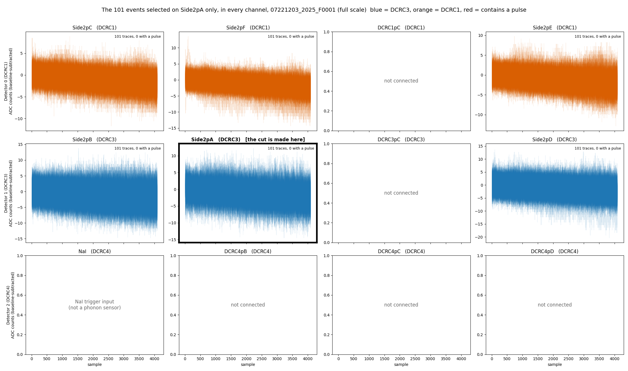
Figure 8: The 101 randoms that pass the cut on PAS2, in every channel, at full scale. The cut is made on PAS2 (framed). One tile per channel, with the traces drawn over each other with transparency, baseline-subtracted. Blue is DCRC3 and orange is DCRC1; no trace contains a pulse. The 6 tiles with grey text are the inputs that are not sensors.
Appendix C: both faces of the detector
The detector has two faces with the same six phonon sensors each (A
the outer ring, B the second ring, C, D and E the three sectors of the
middle region, F the centre disc). In the Side-2 readout of this series
only the sensors of Side 2 are connected to a readout board, so Figure 1
shows one face. Figure 9 draws both: Side 2 as in Figure 1, and Side 1,
which is not read out, greyed out and labelled with the board input each
of its sensors would use in the Side-1 readout of the same Setup table.
The drawing is made by detector-faces-buddy.ipynb
from python/pulse_channels.py
(sensor_channels(readout=2) and
sensor_channels(readout=1)).
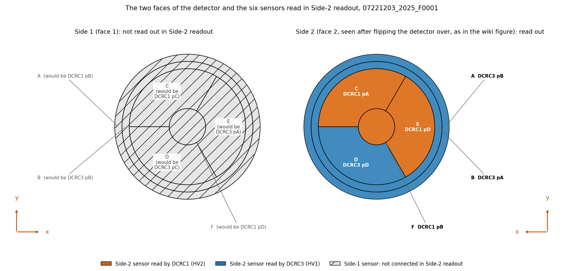
Figure 9: Both faces of the detector S104 and the six sensors read in the Side-2 readout. Left: Side 1 (face 1), not read out in this series (hatched; the board inputs in grey are those of the Side-1 readout, which this series does not use). Right: Side 2 (face 2, seen after flipping the detector over, as in the wiki figure), with each sensor coloured by its readout board, DCRC1 (orange, HV2) or DCRC3 (blue, HV1), and labelled with its letter, board and input, as in Figure 1.