Noise-pulse selection on Detector 0 / Channel 0 (series 07221203_2025, dump 1)
Code Repository
Notebooks and library files this note rests on, each pinned to the commit that produced the results below:
07221203_2025_dump1_noise.ipynb— the main notebook for everything below. Pinned to1958479.dump1_noise_pulses.ipynb— the original first-pass notebook, superseded but kept for history. Pinned toc892af4.python/— the pulse library the notebook now uses (see Note 1a). Pinned to085aa3d.
Goal and setup
Pick out clean noise traces on Detector 0, Channel 0 of series 07221203_2025, dump F0001 (Run76: Side2, PuBe, Pb&poly lead stack and borax, −83.2 V), as the input to a noise-PSD study. The dump has 4551 channel groups; Detector 0 / Channel 0 contributes 1517 traces of 4096 samples each.
Definitions
Let xi be sample i of a trace (i = 0 … 4095, in ADC counts), N the length of the pretrigger window (1000 or 500 samples; both are compared below), and g = 10 the number of leading glitch samples that are skipped.
| Quantity | Definition | Library function |
|---|---|---|
bmean | Mean of xi over the pretrigger window, i = g … N−1 | pretrigger_mean |
bstd | Standard deviation of the same samples (population form, divisor N−g) | pretrigger_std |
dev | Largest deviation from the baseline after the pretrigger window, either polarity: max over i = N … 4095 of |xi − bmean| | max_deviation |
ratio | dev / bstd | excursion_ratio |
log10(ratio) | Base-10 logarithm of ratio, the quantity plotted and cut on throughout this note (a trace with dev = 0 would give −∞ and is excluded; none occur here) | log_excursion_ratio |
ratio is dimensionless: it is the size of the trace’s largest post-pretrigger excursion measured in units of the trace’s own baseline scatter, so it does not depend on the overall scale of the trace. A large ratio means something after the pretrigger window stands well above the baseline noise (a pulse, a drift, or simply the largest noise fluctuation); what values to expect for pure noise, and what a small ratio means, is worked out in “First cut, and why it is misleading” below.
Some traces have a brief (1–5 sample) electronic step glitch at the very start, which is why the first g = 10 samples are skipped in bmean and bstd. That fixes the glitch but not a real pulse that reaches into the pretrigger window.
dev is measured only after the pretrigger window on purpose. Measuring it over the same samples that set bstd puts a hard floor near ratio ~ 1 whatever threshold is used, which made an initially requested threshold of 0.5 impossible to reach.
First cut, and why it is misleading
The first “good noise” cut kept traces with bstd below its own 75th percentile and ratio below its own 25th percentile (bstd < 32.48, ratio < 1.93): 41 of 1517 traces. Plotting log10(ratio) for all traces shows two features: a sharp spike near 0 and a broad hump from about 0.5 to 1.4.
Not to be confused with the 21-trace good_noise_traces.csv selection that feeds Note 3: that comes from the original notebook, with different scope, thresholds and baseline definition, and shares no events with these 41. Note 3 compares the two.
Repeating the calculation with the pretrigger window shortened from 1000 to 500 samples changes the picture:
- the near-zero spike disappears;
- the broad hump stays where it was, so it does not depend on the window length;
- a new bump appears near
log10(ratio)2.0–2.4: pulses that start between sample 500 and 1000 are correctly seen as excursions with the shorter window, but were swallowed into the baseline with the longer one.
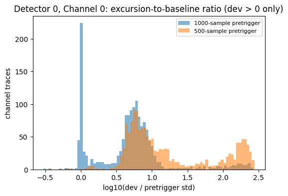
log10(dev/bstd) for Detector 0 / Channel 0, 1000-sample window vs. 500-sample window overlaid. The near-zero spike exists only with the 1000-sample window.The reason is extreme-value statistics. dev is the maximum over roughly 3000 samples, so even pure Gaussian noise lands around ratio ~ 3–8 (log10 0.5–0.9), not near 1. A trace only reaches ratio ~ 1 if its own bstd is inflated, i.e. its pretrigger window already contains part of a pulse or a slow drift. The low-ratio spike is contamination, not quiet noise — the naive “smaller ratio means quieter” expectation is backwards.
Branch 1: the 1000-sample window
Widening the near-zero slice to log10(ratio) in [−0.05, 0.48) gives “Cut A” (417 traces); the broad hump [0.5, 1.0) on the same window gives “Cut B” (892 traces).
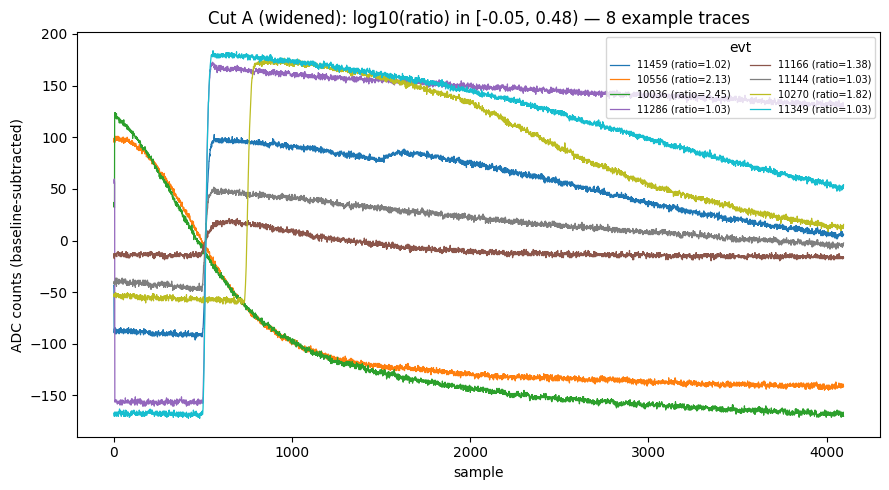
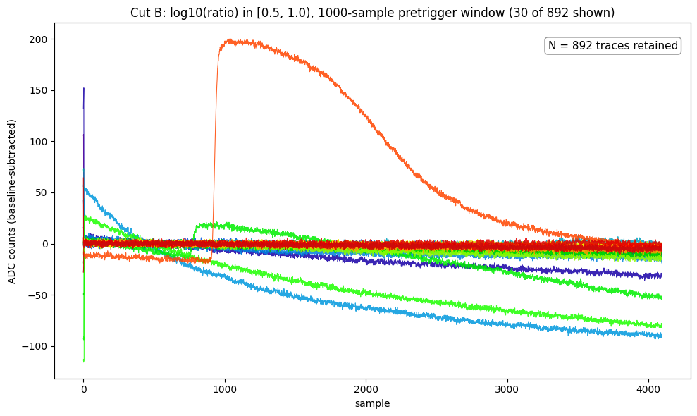
pulse_quantities.rise_sample, a half-maximum-crossing heuristic that is tagged under_development and has only been used on this one analysis. Treat it as a working hypothesis. In the notebook this section is collapsed by default and carries the same warning.
Hypothesis: if the Cut A pulses have similar amplitude, then the later a pulse rises, the less of the pretrigger window it contaminates, so bstd is smaller and ratio larger. Estimating a rise sample per trace (first post-pretrigger sample crossing half of dev) over all 417 traces gives a Pearson correlation of 0.45 between ratio and rise sample, with rise samples spanning 1000–2698. The scatter has two components: a floor at exactly 1000 (pulses that already crossed half-maximum inside the pretrigger window, so the method reports the window boundary), and a genuine rising trend above it (ratio 1.3–2.9 with rise sample 1200–2700). Consistent with the hypothesis, but not independently verified.
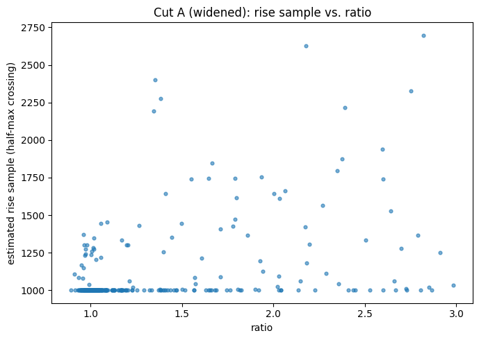
ratio; correlation 0.45. Unverified — see the warning above.Branch 2: cut on the 500-sample window
Instead of refining Branch 1, cut directly on the clean hump of the 500-sample window. All of these use the 500-sample pretrigger window and dev > 0.
| Cut | Window | log10(ratio) | Traces (of 1517) |
|---|---|---|---|
| “Good noise” (first cut) | 1000 | bstd < 32.48 (p75) and ratio < 1.93 (p25), i.e. log10(ratio) < 0.29 | 41 |
| Cut A (widened) | 1000 | [−0.05, 0.48) | 417 |
| Cut B | 1000 | [0.5, 1.0) | 892 |
| Branch 2 | 500 | [0.5, 1.4) | 1012 |
| shoulder | 500 | [1.0, 1.4) | 268 |
| high tail | 500 | ≥ 2.0 | 346 |
| Loose | 500 | [0.5, 1.0) | 744 |
| Tight | 500 | [0.5, 0.7) | 192 |
Cut B and Loose cover the same log10(ratio) range, [0.5, 1.0), but on different pretrigger windows: Cut B uses 1000 samples (892 traces), Loose uses 500 (744 traces). Within Branch 2, Loose is the wider of two narrowed cuts: it stops short of the shoulder, [1.0, 1.4), where contamination starts creeping in, but keeps the most traces. Tight, [0.5, 0.7), is narrower still and cleaner, at the cost of statistics. They are the library’s excursion_band_loose and excursion_band. Neither is claimed to be the ideal noise selection; the names only say how wide the slice is.
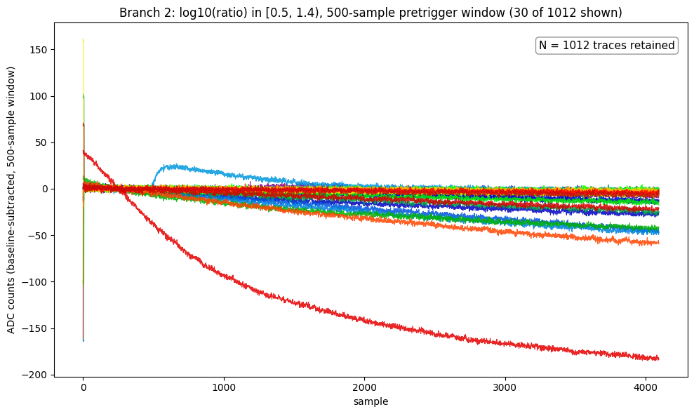
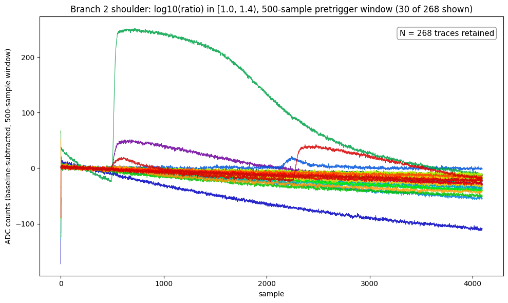
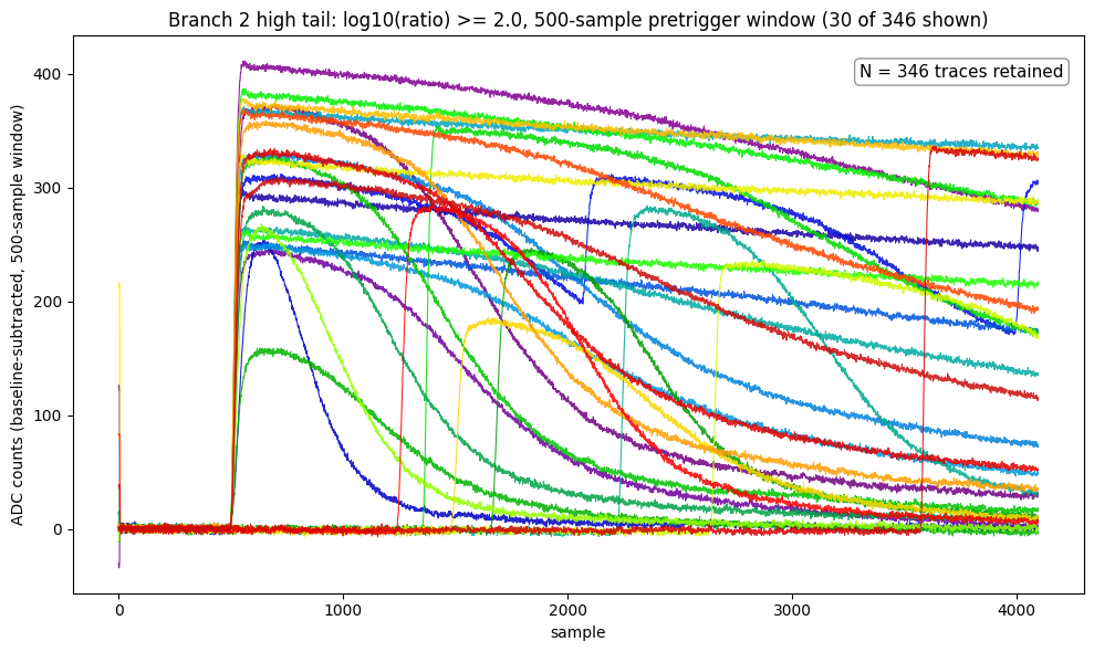
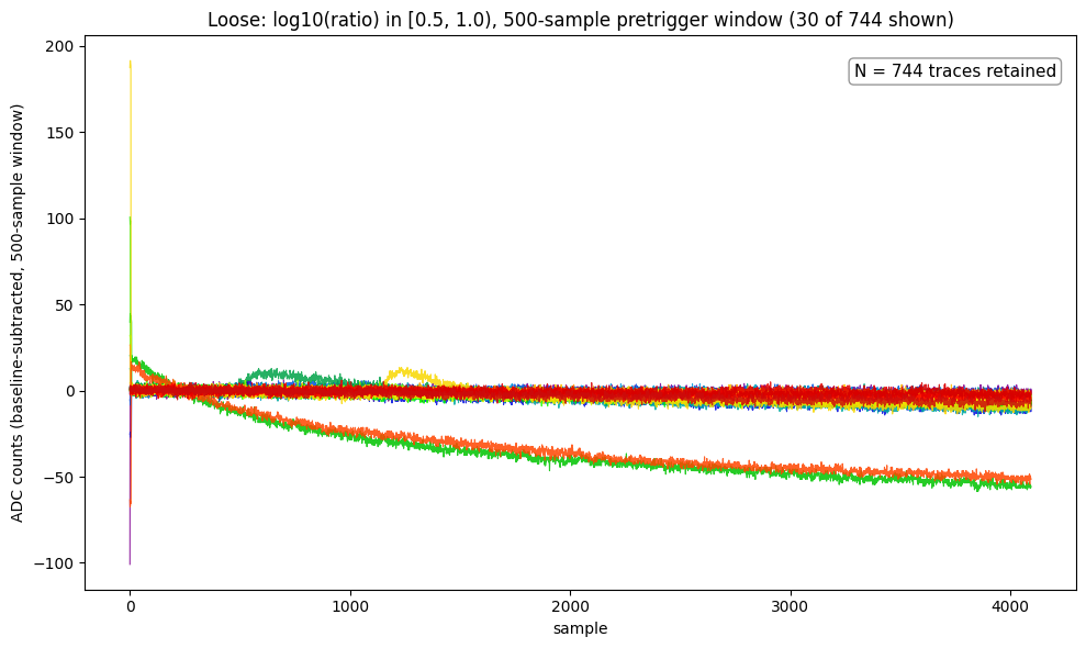
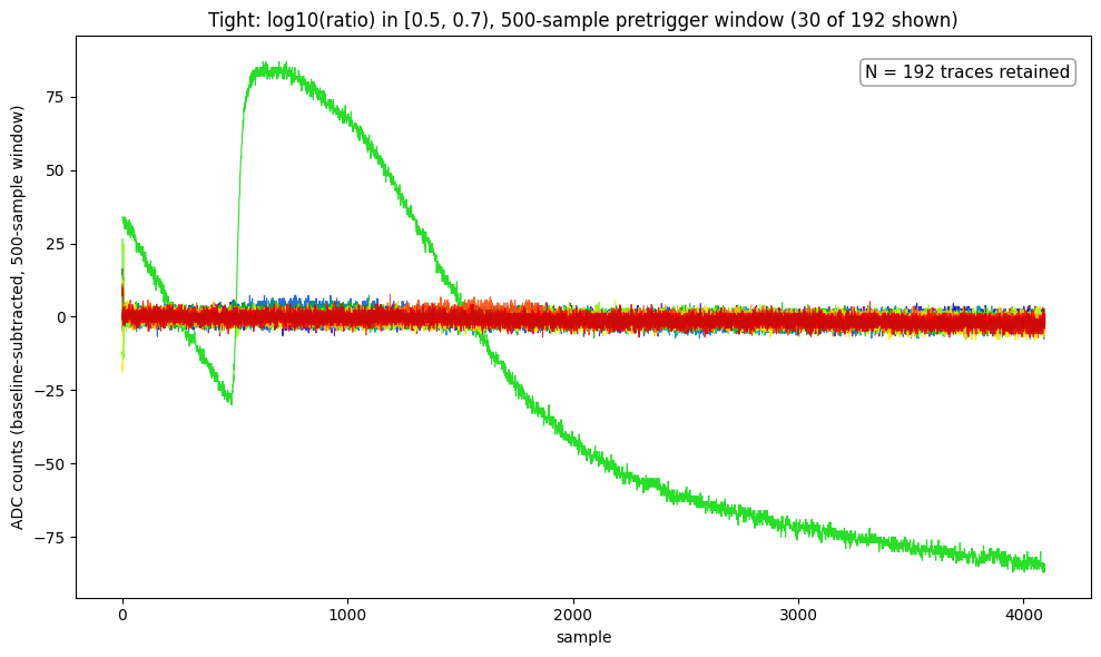
Moving down in ratio makes the selection cleaner: contamination increases toward the shoulder, and the high tail is real pulses. The Tight slice is the cleanest, but even it lets a few real pulses and drifts through: 13 of its 192 traces, called “the 13 pulse-like traces” below. Note 6 describes how they were identified (by pulse shape).
Restricting bstd in Branch 2
Branch 2’s cuts so far look only at ratio. The first cut of this note also capped bstd (bstd < 32.48, the 75th percentile of the 1000-sample bstd). Applying the same number as a cap on Branch 2’s own 500-sample bstd, on top of the Tight cut, keeps 189 of the 192 Tight traces (and 738 of the 744 Loose ones). The plot below shows the same 30 traces as the Tight plot above, minus any the cap removes; none of the three removed traces were in that sample, so it looks the same.
Does the cap remove the obvious green trace? No. That trace (event 11539: a baseline decaying from about +33 to −30 across the pretrigger window, then a pulse rising near sample 500) has a 500-sample bstd of 18.05, well under the cap, so it is kept. The three traces the cap does remove have bstd of 33 to 72: two large drifts and one large pulse.
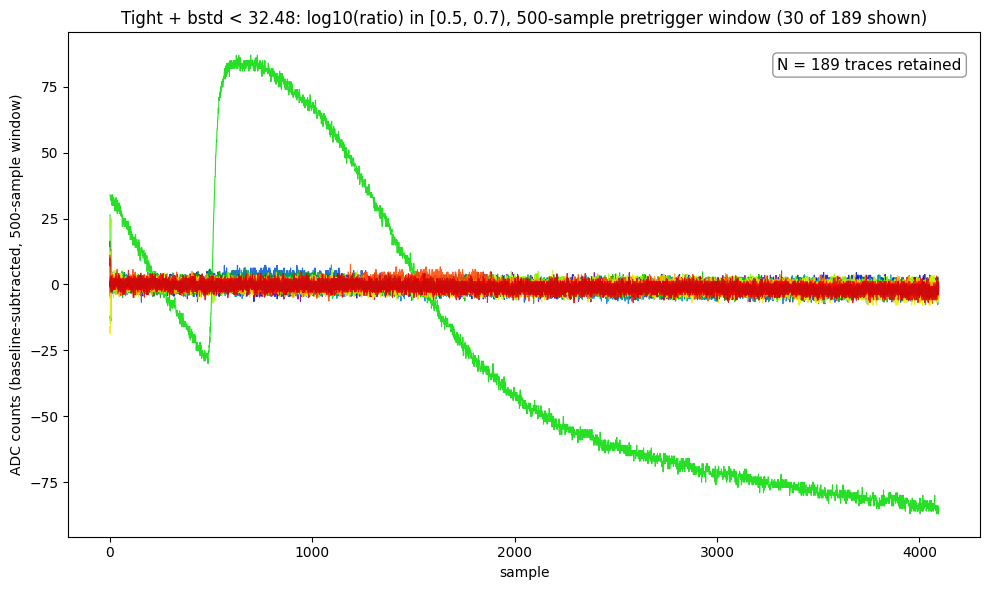
bstd < 32.48: 189 traces (30 shown, the same sample as the Tight plot). The large green trace is still there.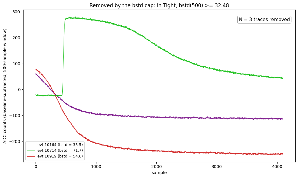
Histogram of bstd for the 500-sample window
We use the plot below to see whether adjusting the bstd cut is worth it: a bstd threshold can only help if the traces we want to remove sit apart from the ones we want to keep. It shows all Detector 0 / Channel 0 traces (1517) as a histogram of log10(bstd) on the 500-sample window, with the Tight selection overlaid in orange, the 1000-sample bstd as a black outline for comparison, and the 32.48 cap as a dashed line. The count axis is logarithmic because the quiet population dominates and the interesting part is the tail.
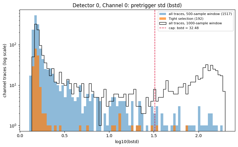
log10(bstd), Detector 0 / Channel 0: all 1517 traces on the 500-sample window (blue), the 192 Tight traces (orange), the 1000-sample window (black outline), and the 32.48 cap (dashed). Log count axis.| Window | p50 | p75 | p90 | p95 | p98 | max |
|---|---|---|---|---|---|---|
| 500-sample | 1.54 | 1.69 | 3.42 | 10.53 | 33.39 | 179 |
| 1000-sample | 1.88 | 32.48 | 124.91 | 149.76 | 170.51 | 199 |
500-sample bstd | All traces | In Tight |
|---|---|---|
| 0 to 2 | 1249 | 175 |
| 2 to 5 | 158 | 5 |
| 5 to 32.48 | 78 | 9 |
| ≥ 32.48 | 32 | 3 |
The 500-sample bstd is sharply peaked near 1.5 (median 1.54; 1249 of the 1517 traces are below 2) with a sparse tail out to 179. The 1000-sample bstd (black outline) has a second population at bstd of roughly 80 to 180 (log10 about 1.9 to 2.25): the pulse-contaminated baselines discussed above, pulses that start between samples 500 and 1000. That population is why its 75th percentile is 32.48 and its 90th is 125. It is largely gone in the 500-sample window (32 traces, 2%, at or above 32.48), so the same number that sat in the valley between the two populations for the 1000-sample window now sits in a sparse tail.
A separate bstd cut: log10(bstd) < 0.5
We add a separate cut on the baseline scatter alone, independent of ratio: log10(bstd) < 0.5 on the 500-sample window. The quantity being cut on, log10(bstd), is the horizontal axis of the histogram above; in terms of bstd itself, it selects traces with bstd below 3.16 (100.5). On its own, this cut keeps 1355 of the 1517 traces (89%). When applied after the Tight cut, it keeps 179 traces and removes 13. The plot shows the same 30 traces as the Tight plot above, minus the one that this cut removes, so the two compare directly.
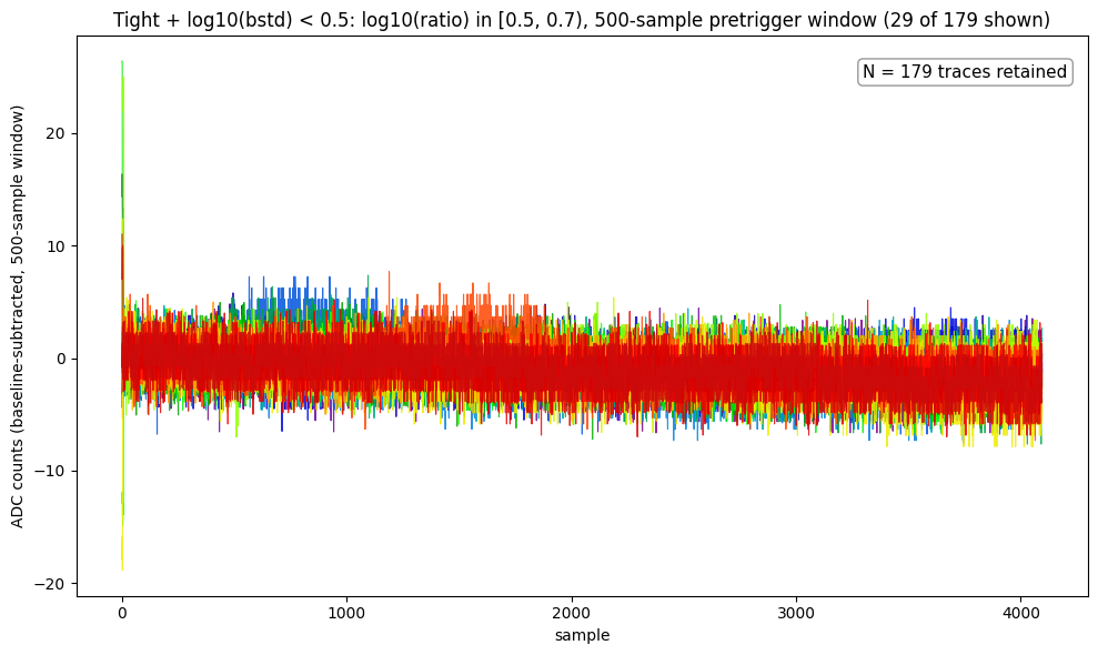
log10(bstd) < 0.5: 179 traces (29 shown: the Tight sample minus the one trace removed). Compare the Tight plot above.The large green trace of the Tight plot (event 11539, bstd 18.05) is removed. What is left in the sample is flat noise with no pulses or drifts; a few traces show brief stretches of somewhat larger scatter, up to about 7 counts. The 13 removed traces are exactly the 13 pulse-like traces, and the 179 retained are exactly the rest of the Tight cut (checked in the notebook). The 13 were identified in Note 6 from their pulse shape, not from their baseline scatter.
The exact match is a meaningful agreement between two different criteria, though not a full test of the bstd cut. The threshold 0.5 was chosen from the histogram alone, where the distribution starts to rise sharply, without reference to the pulse-like traces, and it removes exactly the 13 that were identified from their pulse shape. The match is also not sensitive to the exact value: among the Tight traces, the 179 that are not pulse-like have bstd up to 2.83 and the 13 pulse-like traces start at 4.65, so any threshold in that gap, 3.16 included, gives the same result. It is not a full test because the pulse-like classification is itself a heuristic, and because this is one detector and channel: it shows that baseline scatter alone separates the two groups within the Tight cut, not that the cut would work on another selection.
Applied to the Loose cut, the same bstd cut removes 53 of the 744 traces (691 kept); how many of those 53 are pulse-like has not been checked.
Status / Next Steps
- The Tight cut is now a library function (
excursion_band), and the Loose cut isexcursion_band_loose; see Note 1a. - The 13 pulse-like traces in the Tight selection are identified and removed in Note 6.
- The rise-time hypothesis (Branch 1) is still unverified;
rise_sampleneeds checking against noisy and multi-peak traces first. - Everything here is one detector and one channel of one dump. Other channels and other dumps have not been done (Channel 2 was 100% dead in this dump, so it needs a separate look).
- The cut boundaries (0.5, 0.7, 1.0, 1.4) were chosen by looking at plots, not derived from a model of the noise.
- Choose the
bstdcap for Branch 2: 32.48 is loose in the 500-sample window, and any value between 2.83 and 4.65 (the largestbstdamong the Tight traces that are not pulse-like and the smallest among the 13 that are) removes exactly the 13 pulse-like traces on this dataset. But the overall 500-samplebstddistribution has no natural break between about 2 and 30 (see the histogram), so the value needs another justification. The next attempt,log10(bstd) < 0.5, was chosen from the histogram alone and removes exactly those 13 from the Tight cut. It has mostly been examined on the Tight cut.