−Table of Contents
Review of Python ML Clustering Algorithms
Complete SciKit-Learn Documentation. Read this for in depth knowledge.
Intel(R) Extension for Scikit-learn. Speeds up default algorithms by patching functions.
Apply sklearnex with:
from sklearnex import patch_sklearn
patch_sklearn()
A review of 10 different clustering algorithms was performed to evaluate their effectiveness to automatically group position event clusters in SCDMS data. If an effective algorithm could be found it would speed up the analysis time by automating the event selection cuts, as well as improve the accuracy of cuts by selecting exact clusters of desired data instead of manual linear cuts that leave behind a few noise points.
All algorithms used are available as part of the python scikit-learn:
conda install -c conda-forge scikit-learn
Data used for testing: \\shi\\k100proc\\midasrq\\byseries\\07201024_1012
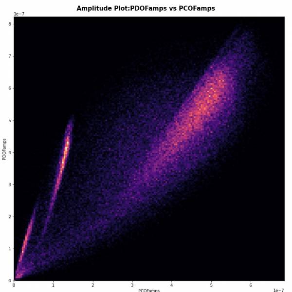
The clearest visual clusters appear in a PCOFamps vs PDOFamps mapping, so all tests are performed on these rqs.
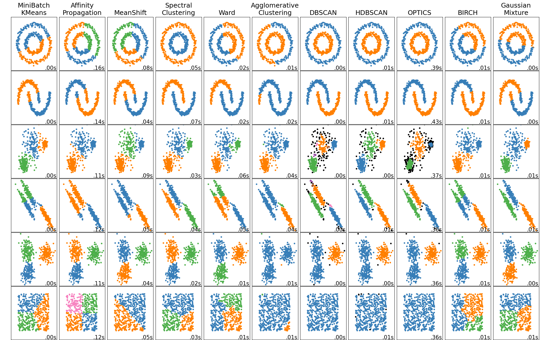
Choosing the right parameters for the algorithm are very important for determining the length of time it takes to process. Normal calculation times should take less than a minute if done effectively. During testing I started with the wrong values, while testing input ranges for parameters, and the calculation would take 3+ hours or never end which would require a hard restart of jupyterlab or even computer. For some algorithms, they can not handle our large datasets (~100k values) so smaller samples were tested for evaluation in the ~500-1000 range. If any of these algorithms show promise, then the data would have to be fully processed in a small batch mode.
Algorithms tested:
- Affinity Propagation
- Agglomerative Clustering
- BIRCH
- DBSCAN
- K-Means
- Mini-Batch K-Means
- Mean Shift
- OPTICS
- Spectral Clustering
- Mixture of Gaussians
Values used for important relevant variables to produce shown plots are given below in each section
Conclusion:
DBSCAN is the most effective since it works purely on a density approach for analyzing our noisy data plots. I wonder if there is a different way to plot the data that would shape clusters into more circular blobs easier for algorithms to distinguish. Multiple manual cuts still seem the most effective at this point.
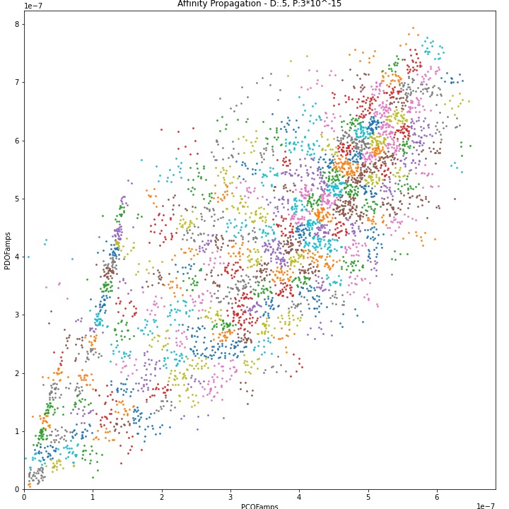
Affinity Propagation
Robust explanation of affinity propagation
Batch Size: 5000
damping: 0.5
preference=-(3*10**-15)
Result: Affinity propagation is poorly suited to large datasets, as it's calculations involve large matrices with computations scaling to N^2 where N is length of data. I ran at a moderately sized 5000 length and required extreme fine tuning of the preference parameter for any clusters to appear. The preference parameter is calculated as = - (distance between points)^2. I estimated what I wanted to start and then had to progressively narrow down my search, as slightly too small will make too many clusters, or if pref=0 then n_clusters will equal batch size, ie 5000. If preference is set too large then a single cluster will be found.
Agglomerative Clustering
Batch Size: 40,000
n_clusters=20
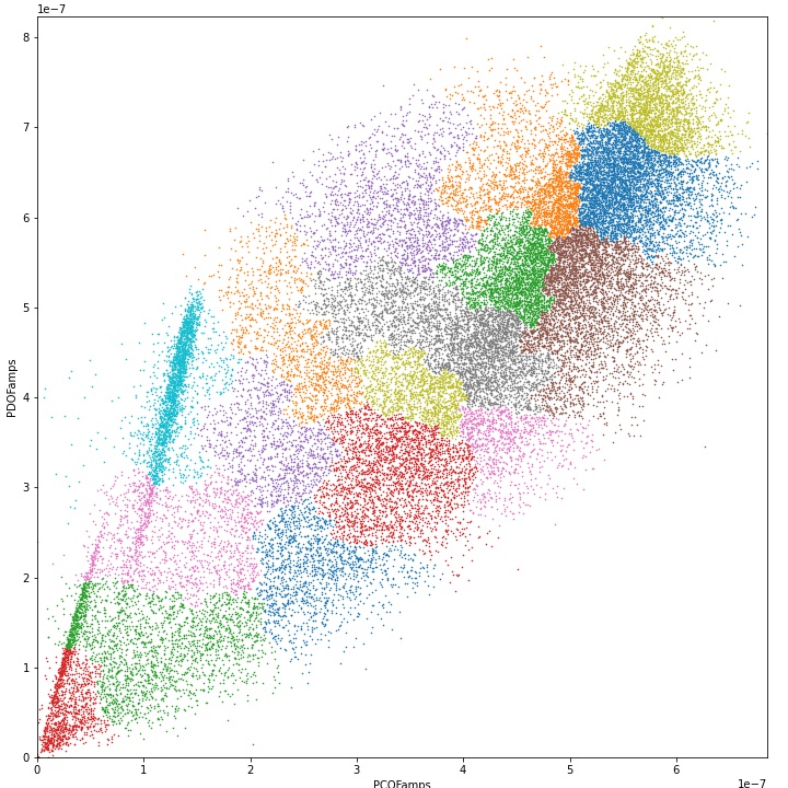
Result: Unable to locate clusters.
BIRCH (Balanced Iterative Reducing and Clustering using Hierarchies)
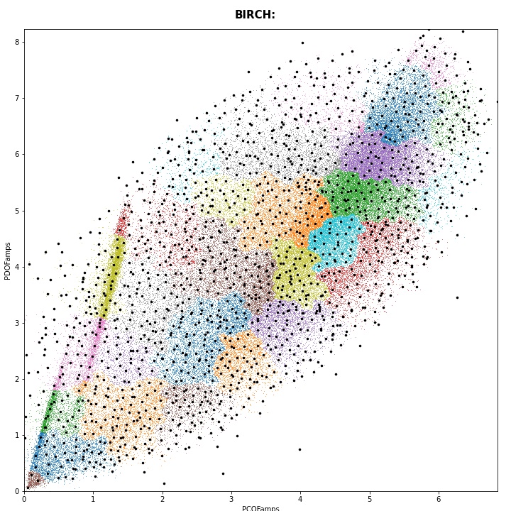
Batch Size: 108,000
threshold=.1
n_clusters=30
branching_factor=10
Results: This plot may look extreme, but it is exaggerated for an explanation. BIRCH works by grouping subclusters into larger clusters. So each dot represents the centroid of each subcluster, and on certain edges, you can see the shape of the subclusters. This method also fails at low cluster counts and higher thresholds. Noise and shape is still a problem.
DBSCAN (Density-Based Spatial Clustering of Applications with Noise)
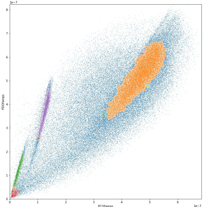
Batch Size: 108,000
eps=5*10^-9
min_samples=80
Results: Found good clusters. Results highly dependent on relation between variables. Small variations in either distance while keeping minimum constant or variations in minimum with distance constant will cause large differences in clusters. Too high or too low will group everything as 1 cluster or ignore everything. A reasonable best clustering was found below. It is difficult to find the balance so the desired cluster does not get group with the high density blob emanating from origin.
K-Means
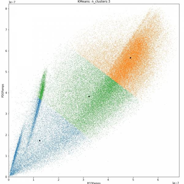
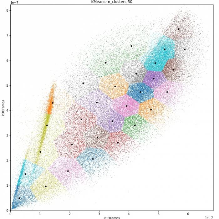
Voronoi diagrams. KMeans tries to cluster data based on centroids while minimizing “within-cluster sum-of-squares”. Even when algorithm was given initial centroid locations with 1 pass, it ignored to evenly distribute off initial points. Could not figure out how to make it not recalculate centers.
Batch Size: 108,000
n_clusters=3, 30
n_init=20
random_state=0
Results: Not useful for noisy, non-circular data clusters. Appears to sort into basic evenly sized groups.
Mini-Batch K-Means
Batch Size: 108,000
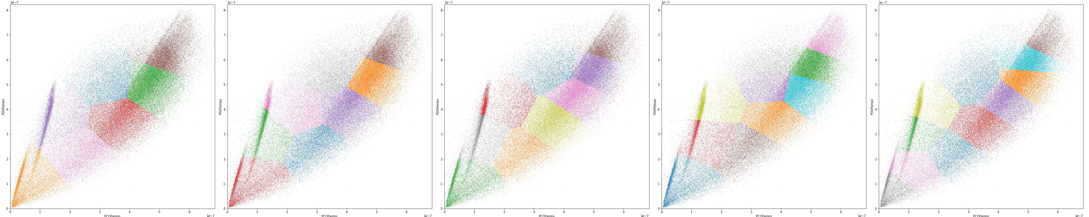
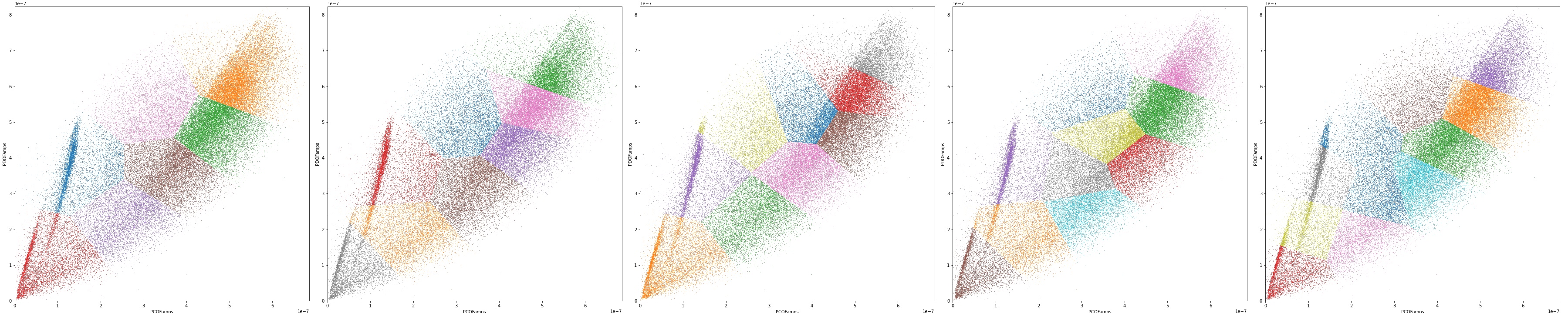
n_clusters=2-11
Results: Unable to to identify clusters.
Mean Shift
Batch Size: 108,000
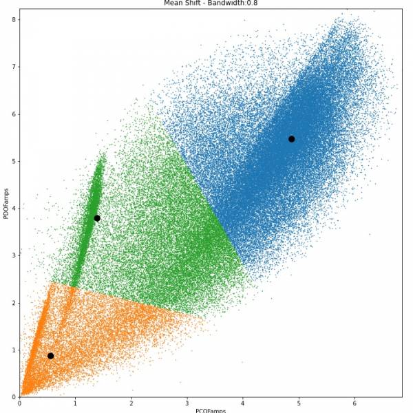
bandwidth = estimate_bandwidth(ta, quantile=0.1, n_samples=10000)
bin_seeding=True
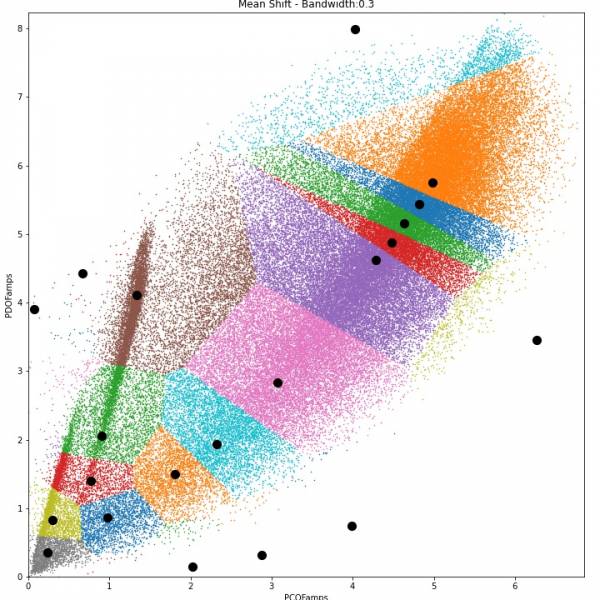
Results: Mean shift tries to detect centralized blobs, so was not a good match for our data. PDOFamps & PCOFamps values are *10^7 for ease of plotting and to prevent possible errors with numbers too close to zero. Centroids of the MeanShift algorithm are plotted as black circles. The centroids are fairly well identified for our clusters, but MeanShift has no way to ignore the numerous noise in our data.
OPTICS (Ordering Points To Identify the Clustering Structure)
Batch Size: 20,000
eps=1*10^-6
min_samples=10
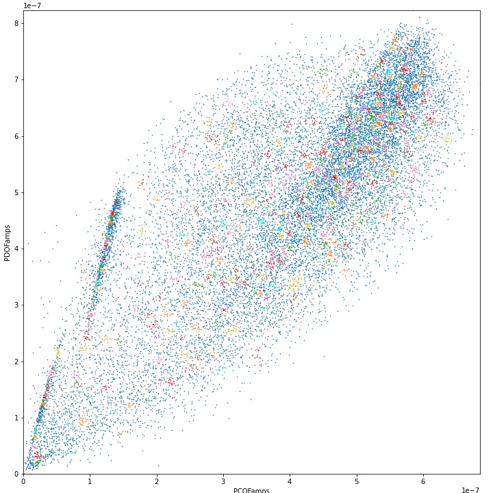
Results: OPTICS seemed to form small clusters at random in high and low density regions.
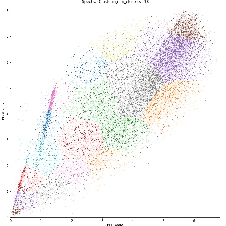
Spectral Clustering
Batch Size: 20,000
n_clusters=18
eigen_solver='amg'
assign_labels='kmeans'
random_state=0
gamma=1.0
Results: Results no better than other clustering algorithms used so far. Possibly because it is built on KMeans? Spectral required a small batch size to compute efficiently even when using the more efficient pyamg package for computing eigenvectors. Spectral is one of the more complex algorithms used, and it may still be possible to achieve better results with better kwargs.