Comparison of all four SiPM
Each SiPM was run with a 1.806kOhm resister in order to make sure that photoelectron peaks are visible in each histogram.
Short Runs
Short run (10k events) files:
130708_sipm1_blueled_delayed-trig_10hz_100ns_1.806kOhm.dat
130708_sipm2_blueled_delayed-trig_10hz_100ns_1.806kOhm.dat
130708_sipm3_blueled_delayed-trig_10hz_100ns_1.806kOhm.dat
130708_sipm4_blueled_delayed-trig_10hz_100ns_1.806kOhm.dat
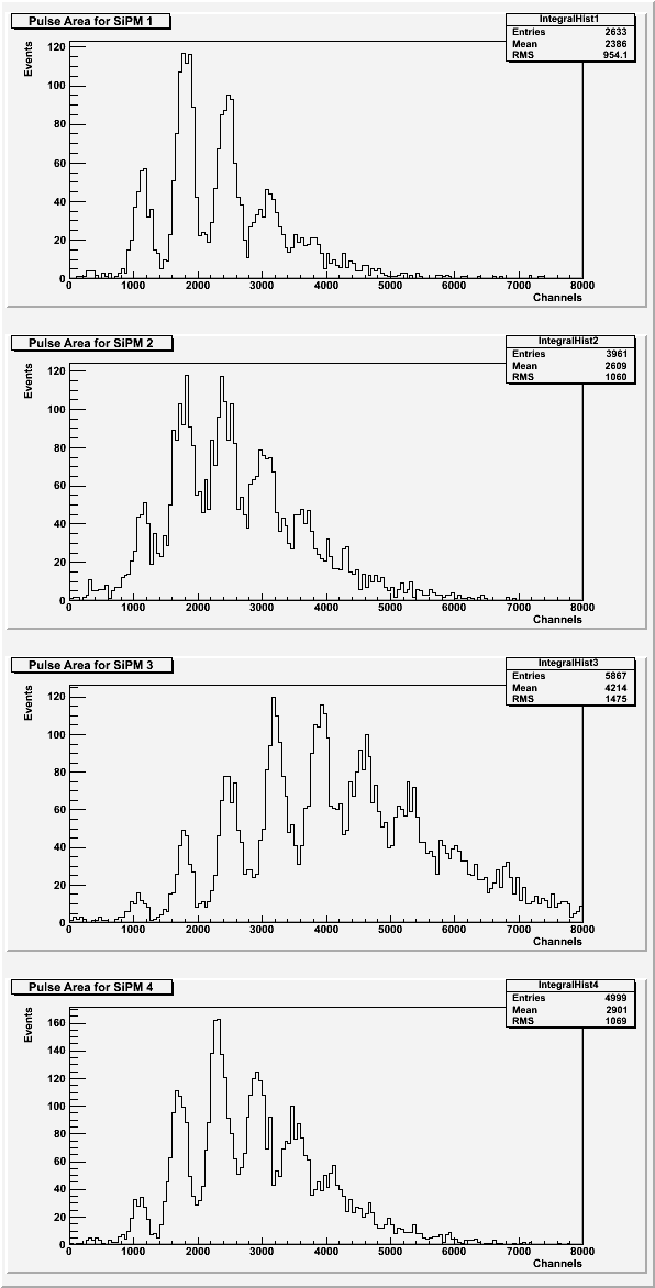
| Figure 1: Area under the pulse for each SiPM. |
 |
| Figure 2: Average pulse maximum for each SiPM. |
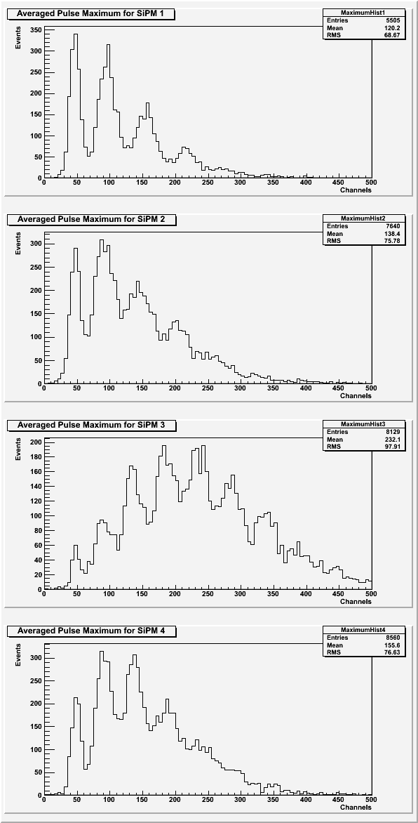 |
For the area under the pulses and the averaged pulse maximum, the photoelectron peaks should look the same for each SiPM. SiPM 3 might have been aligned differently than the other SiPMs to cause a shift in which photoelectron peak has the highest amplitude.
| Figure 3: Rise time of the pulse for each SiPM. |
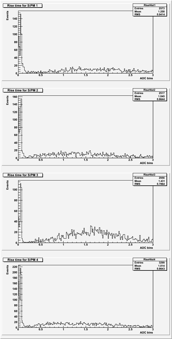 |
Based on previous data sets, the expected rise time for the pulses was around 2 ADC bins. See Rise Time for more details.
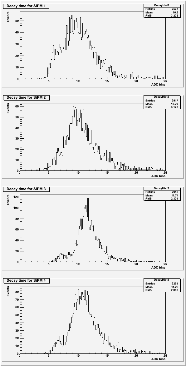
| Figure 4: Decay time of the pulse for each SiPM. |
 |
| Table 1: Description of the cuts for each SiPM. Only data lower than the value given was used. |
| SiPM | Standard Deviation | Chi-squared |
| 1 | 22 | 350 |
| 2 | 25 | 220 |
| 3 | 25 | 190 |
| 4 | 25 | 250 |
The peak area used cuts on the baseline standard deviation and if secondary peaks were present. The averaged maximums used cuts on the baseline standard deviation only. The rise time and decay time used cuts on the baseline standard deviation, the chi-squared of the fit, and on a failure of the fit program.
Long Runs
Long run (100k events) files:
130708_sipm1_blueled_delayed-trig_10hz_100ns_x10_1.806kohm.dat
130709_sipm2_blueled_delayed-trig_10hz_100ns_x10_1.806kohm.dat
130709_sipm3_blueled_delayed-trig_10hz_100ns_x10_1.806kohm.dat
130710_sipm4_blueled_delayed-trig_10hz_100ns_x10_1.806kohm.dat
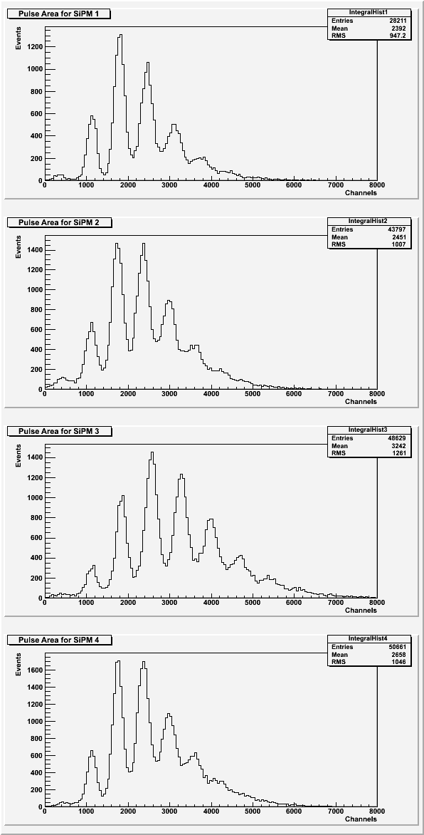
| Figure 5: Area under the pulse for each SiPM. |
 |
| Figure 6: Average pulse maximum for each SiPM. |
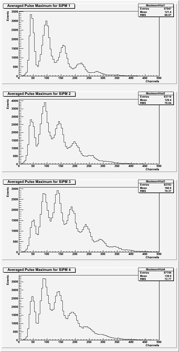 |
Once again, SiPM 3 looks slightly different than the other three SiPMs. Here, however, SiPM looks cleaner. The chi-squared of the fits used for the cut for SiPM 3 is also slightly lower than the other SiPMs (see Table 2).
| Figure 7: Rise time of the pulse for each SiPM. |
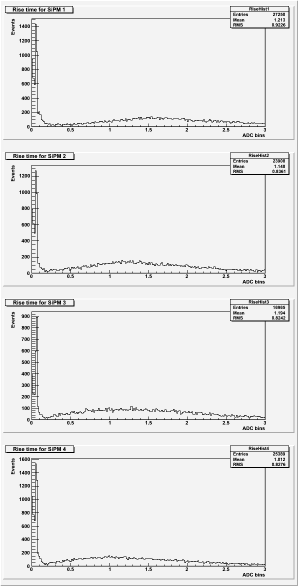 |
Based on previous data sets, the expected rise time for the pulses was around 2 ADC bins. See Rise Time for more details.
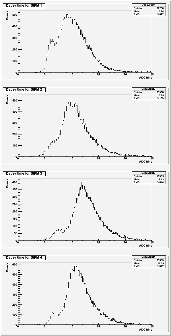
| Figure 8: Decay time of the pulse for each SiPM. |
 |
| Table 2: Description of the cuts for each SiPM. Only data lower than the value given was used. |
| SiPM | Standard Deviation | Chi-squared |
| 1 | 22 | 350 |
| 2 | 27 | 150 |
| 3 | 27 | 120 |
| 4 | 27 | 140 |
The peak area used cuts on the baseline standard deviation and if secondary peaks were present. The averaged maximums used cuts on the baseline standard deviation only. The rise time and decay time used cuts on the baseline standard deviation, the chi-squared of the fit, and on a failure of the fit program.
Rise Time
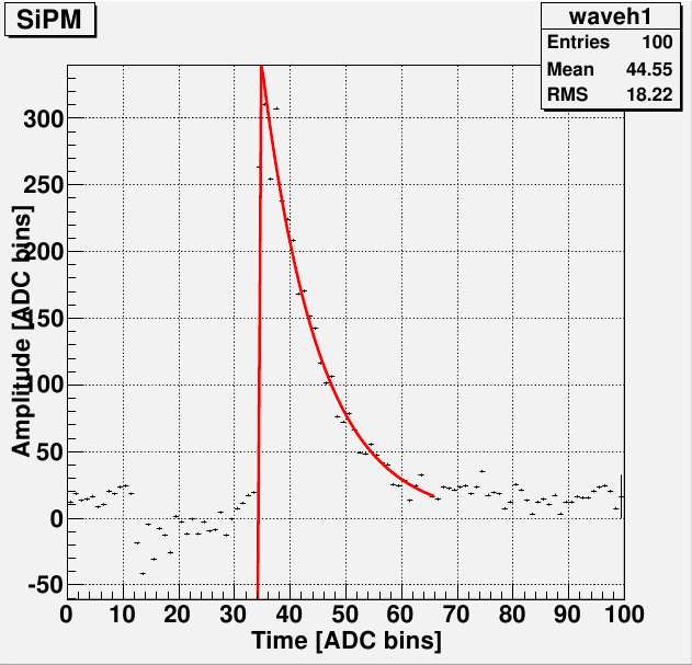
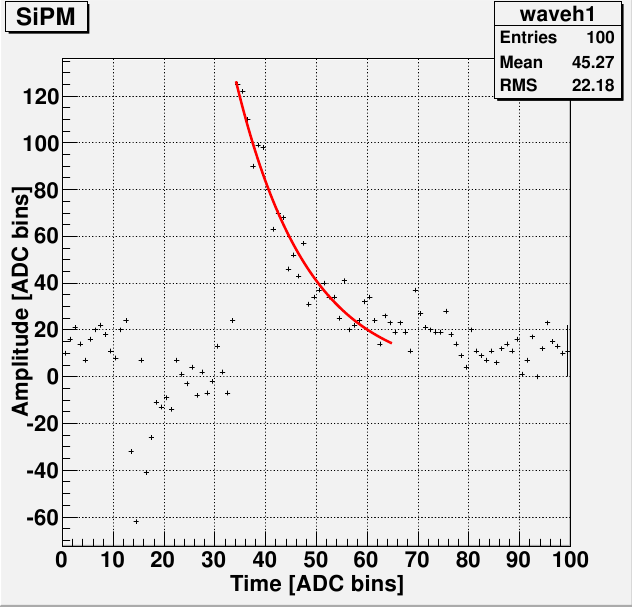
The rise time histograms show rise times to be quite a bit lower than the expected value (2 ADC bins). This appears to be a remnant of double exponential fit. Some pulses do not have enough data points in the rise of the pulse to get a decent fit to that area. This appears to be due to the sample rate of the DAQ and cannot be changed.
| Figure 9: Two examples of pulses with poorly fit rise times. |
 |
 |
| Figure 10: An example of a pulse with an all-around good fit. |
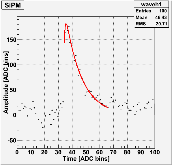 |
The above pulses were taken from the long run of SiPM 1.
Noise in pulse
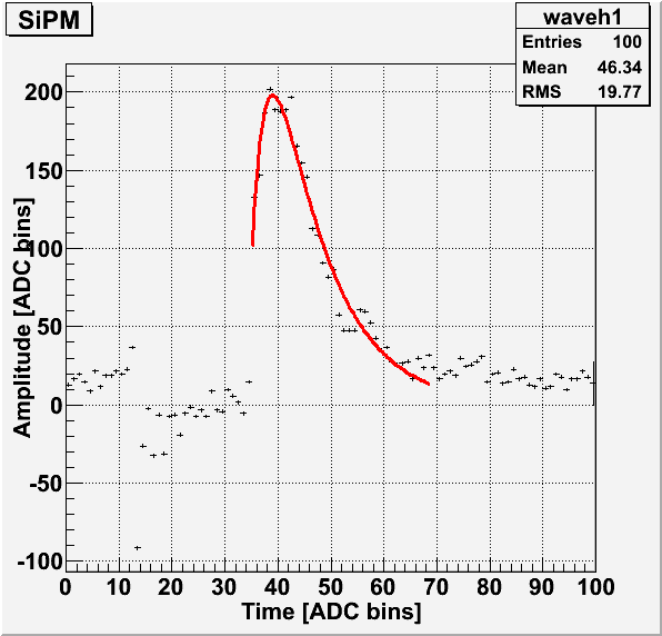
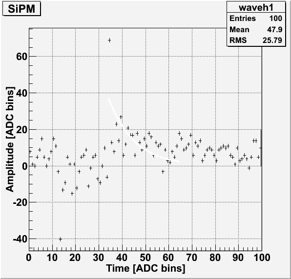
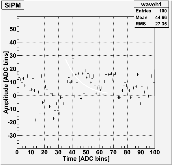
Before the start of each pulse when using the external trigger, there appears to be some sort of noise with a distinct shape. This was thought to be from the trigger, so a 200 ms delay was put in place between the external trigger and when the light pulse and data acquisition begin. This, however, doesn't appear to remove this noise from the pulse.
| Figure 1: Example pulse showing the typical noise just before the start of the pulse for SiPM 1. |
 |
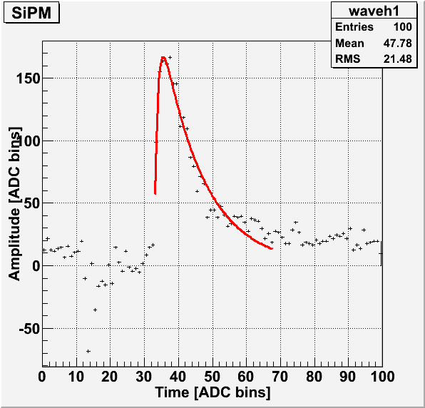
| Figure 2: Example pulse showing the typical noise just before the start of the pulse for SiPM 2. |
 |
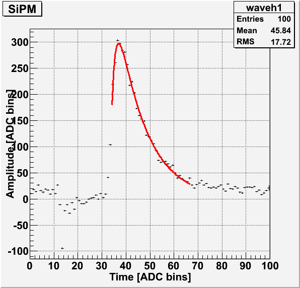
| Figure 3: Example pulse showing the typical noise just before the start of the pulse for SiPM 3. |
 |
| Figure 4: Example pulse showing the typical noise just before the start of the pulse for SiPM 4. |
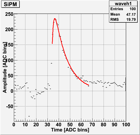 |
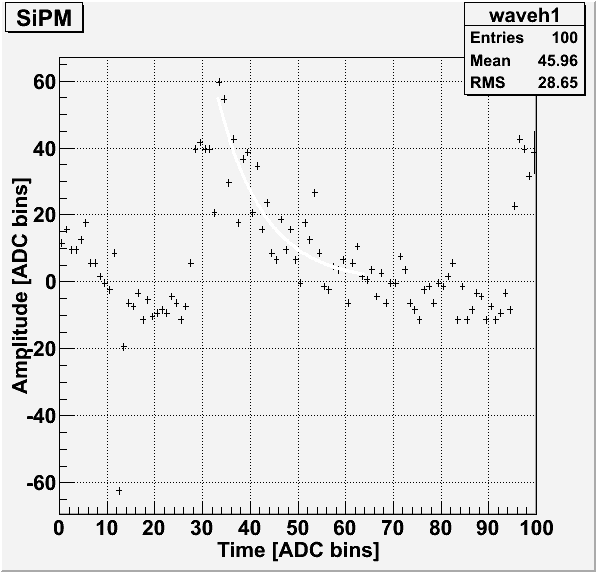
As seen in Figures 1, 2, 3 and 4, the typical shape of the noise is a sharp dip before the start of the pulse. Due to the presence of the pulse, it is difficult to tell if the noise continues into the main pulse. A short run (300 events) was conducted with SiPM 4 with no LED in the dark-box. Each event was externally triggered with a delay of 200 ms. The data file for this run is 130708_sipm4_blueled_delayed-trig-only.dat.
| Figure 5: Four examples of an LED-less run with the same noise visible each time. |
 |
 |
 |
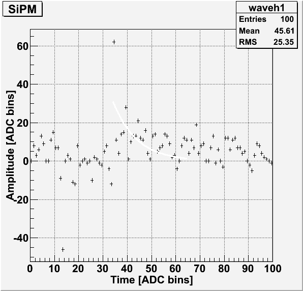 |
In these pulses, there is a sharp peak visible just after the sharp dip. If this is also present in pulses with an LED, this might explain why the pulse area histograms' first photoelectron peak is shifted so far from the origin.
Gain Calculation
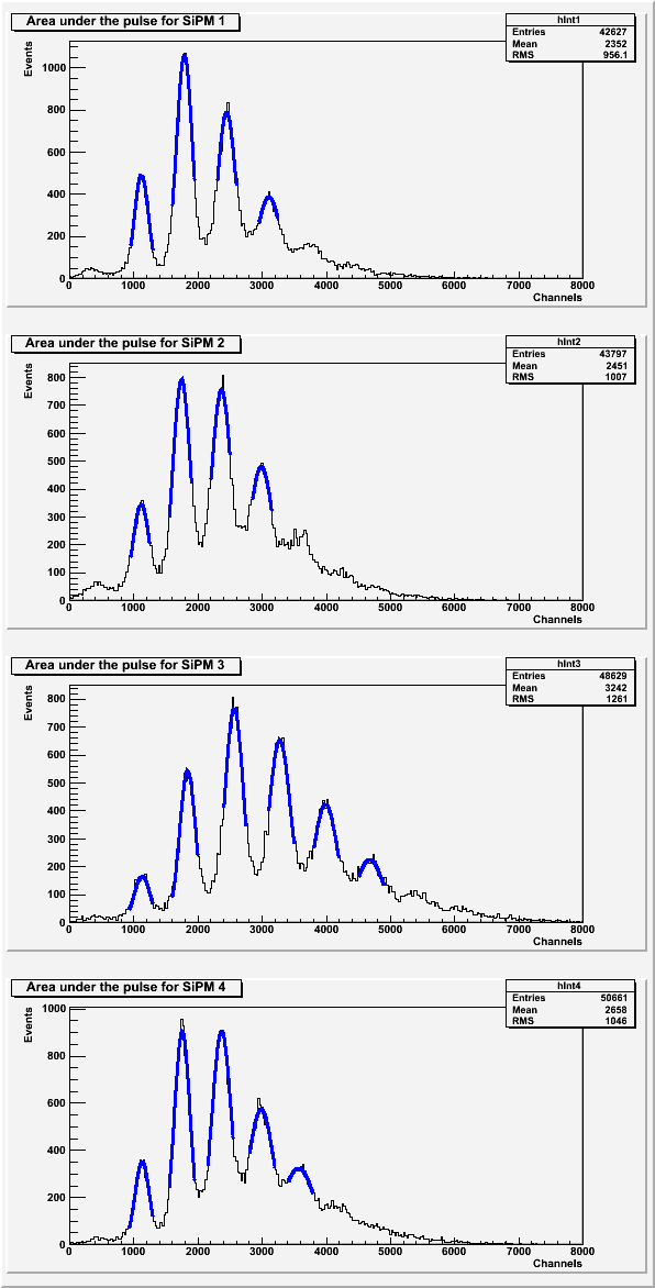
The gain was calculated from the average distance between each photoelectron peak for each SiPM.
| Figure 5: Gaussian peak fits for each photoelectron peak in the area under the pulse for each SiPM. |
 |
| Figure 6: Gaussian peak fits for each photoelectron peak in pulse maximum for each SiPM. |
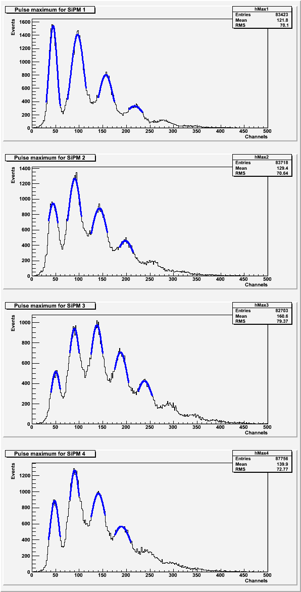 |
| Table 3: Average distance between photoelectron peaks. |
| SiPM | Pulse areas | Pulse maximums |
| 1 | 661.975 | 57.5656 |
| 2 | 623.734 | 51.0148 |
| 3 | 709.109 | 46.9537 |
| 4 | 608.911 | 47.233 |