Pulse height calibration

A wave-generator was connected directly to channel 0 of the DAQ. Square pulses 10 channels wide with varying amplitudes were sent into the DAQ.

Table 1: Data files used.
Run	Amplitude	Data file
1	1 mV	130729_100ns_square-wave_01mV.dat
2	5 mV	130729_100ns_square-wave_05mV.dat
3	10 mV	130729_100ns_square-wave_10mV.dat
4	15 mV	130729_100ns_square-wave_15mV.dat
5	20 mV	130729_100ns_square-wave_20mV.dat
6	25 mV	130729_100ns_square-wave_25mV.dat
7	30 mV	130729_100ns_square-wave_30mV.dat
8	35 mV	130729_100ns_square-wave_35mV.dat
9	40 mV	130729_100ns_square-wave_40mV.dat
10	45 mV	130729_100ns_square-wave_35mV.dat

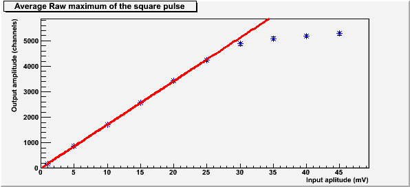
Figure 1: Graph and fit of voltage to channels using maximum amplitude of the square pulse.

The amplitude correction function is:
,
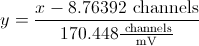where is the amplitude in channels and is the amplitude in mV.

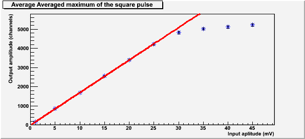
Figure 2: Graph and fit of voltage to channels using average maximum amplitude for the top of a square pulse.

The amplitude correction function is:
,
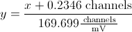where is the amplitude in channels and is the amplitude in mV.

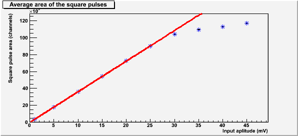
Figure 3: Graph and fit of voltage to channels using the area under the pulse of a square pulse.

The amplitude correction function is:
,
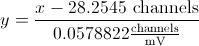where is the area in channels and is the amplitude in mV.

All above fits are not good for pulses with an amplitude greater than around 4500 channels or 27 mV.

Figure 4: Graph of the pulse width for each input voltage.

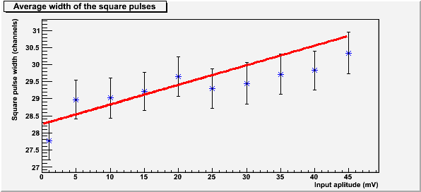The width of the pulses past the saturation limit (~27mV) do not appear to be much greater than the width of the pulses below the saturation limit.

The shown in the above plots (Figures 1, 2, 3, and 4) are one standard deviation. The equation used is shown below.
,
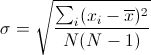where is the standard deviation, is the value of each maximum, is the average maximum, and is the number of maximums used for the calculation.

All calculations for each input amplitude exclude data with a baseline standard deviation greater than 9 (These pulses started within the baseline for some reason).

Figure 5: A typical square pulse.

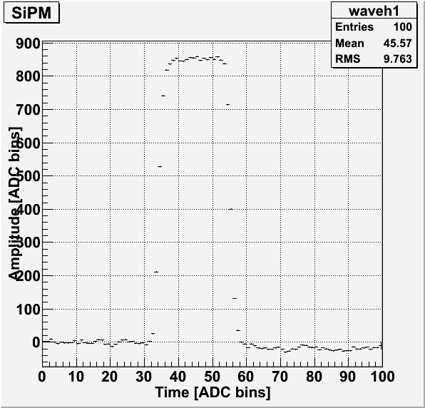The square wave pulse shown in Figure 5 was taken from Run 4 (10mV input pulse).