−Table of Contents
NaI Pulse Shape Analysis
Introduction
The procedure as described here was used. Equation 1 was used to model each pulse shape:
 (1)
To more easily set constraints, Equation 1 was rewritten as Equation 2:
 (2)
where α = A and β = B/A. However, when fitting, fits only behaved when β<0. (I'm not entirely sure why this is the case).
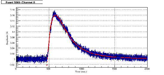
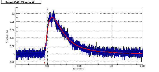
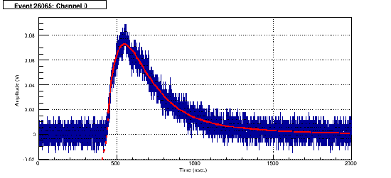
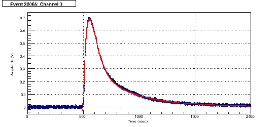
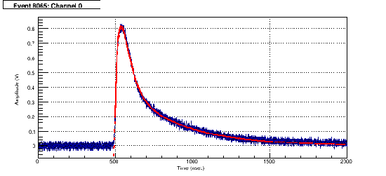
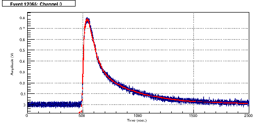
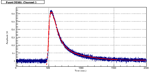
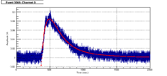
After guessing reasonable initial values for each parameter and setting reasonable ranges, the fits behaved reasonably well, with some exceptions. Fits were done over the range from the time where the voltage was 15% of the pulse amplitude to about 1000 nsec after this point. The bin error was set to be the standard deviation of the pulse baseline. Fits were done using the method of least-squares. Parameter numbers in the ROOT fit equation are as follows:
 (3)
Fit Procedure
Step 1: Determination of Time Constants
File: 20171121_nai_c_anode_1100V_col_75mVthresh_pulseFit2.root Macro: nai_pulseFits.C, nai_pulseFits_analysis.C
τ1 = 99.5 +/- 4.3 nsec
τ2 = 95.6 +/- 4.1 nsec
τ3 = 359 +/- 16 nsec
The parameter to was left free but was constrained to a fairly narrow range (from 400 to 700 nsec), as the pulse did not always start at the same time for each recorded pulse. Per the paper this method was drawn from, α was set to be a positive number and β was set to be a number between 0 and 1.
Examples of Pulse Fits
| Figure 1: | Figure 2: |
|---|---|
 |  |
| Figure 3: | Figure 4: |
 |  |
| Figure 5: | Figure 6: |
 |  |
| Figure 7: | Figure 8: |
 |  |
Data Analysis
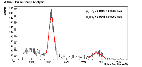
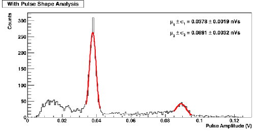
Pulse Amplitude
| Figure 9: Without Pulse Shape Analysis | Figure 10: With Pulse Shape Analysis |
|---|---|
 |  |
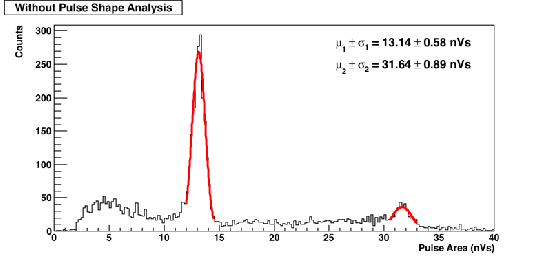
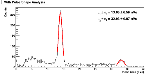
Pulse Area
| Figure 11: Without Pulse Shape Analysis | Figure 12: With Pulse Shape Analysis |
|---|---|
 |  |
By integrating (2) directly, the area under the entire pulse can be calculated using the known parameters using Equation 4:
 (4)