Attenuation Length Study Page 3
I've been looking at a result that seems to be interesting (but expected) on the number of photons generated by the different ways we can simulate muons becoming incident on our scintillator. The three methods:
- Pencil beam (used in all of the attenuation length simulations in the past few meetings)
- square projection (a simple approximation to our trigger system; this is just taking the pencil beam and moving it around a 2×2 grid, but keeping the muon direction constant)
- Simulated trigger (here I used a cos^2 zenith angle distribution, and created an explicit trigger volume to identify valid muon primaries).
I've linked a plot showing the number of photons which were generated by muons under each of these systems:
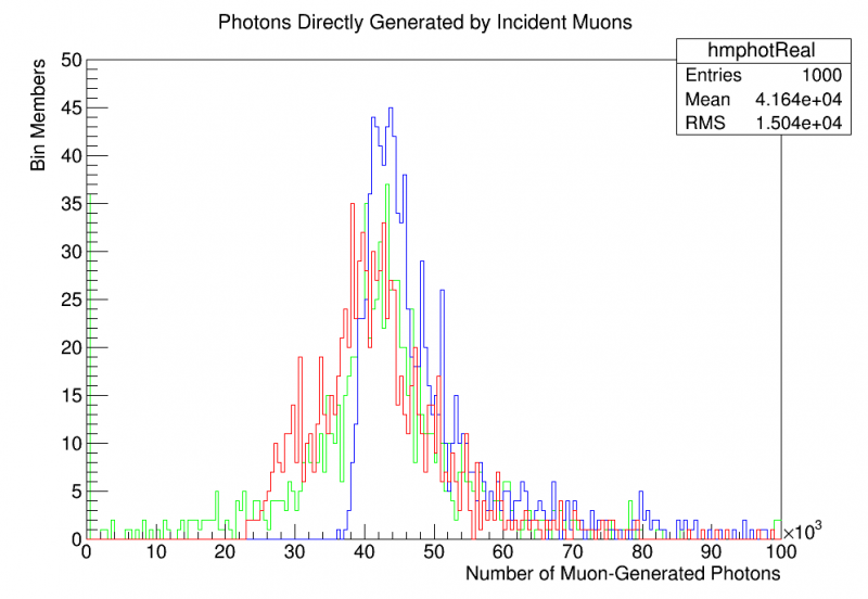
- Blue = Pencil beam
- Red = Square projection
- Green = Simulated trigger
As we can see, the pencil beam creates a clear shift in the average number of photons which are generated by the incident muons as well as in the shape of the spectrum. The previous attenuation length measurements were created using this pencil beam; should we redo this data or is it better to use the pencil beam-generated data?
The square projection and the simulated trigger curves are very close. The simulated trigger seems to be shifted upwards slightly as compared to the square projection, though the two are still statistically consistent under this sample size. It is probably always better to use the simulated trigger since we have it, but the comparison is interesting.
Attenuation Length/Reflection Data Grid
I chose reflectivities of 0.97, 0.98, and 0.99 and bulk attenuation lengths of 0.5 m, 1 m, and 2.5 m (“bulk” = a property of the plastic I assign to it). Using each possible combination of reflectivity and bulk attenuation length, I created measurements at 1,3,5,7,9 cm using the realistic “simulated trigger” muon generation technique. For these events, the “back mask” was simply a PTFE wrapping, NOT a nonreflective black coating. This choice was made because matching the PTFE-backed experimental data is easier than trying to guess what the reflectivity of our black construction paper would be.
For events where a muon triggered, I plotted the number of PE detections then identified the expected number of PE detections for those events. Finally, attenuation length curves similar to the ones seen on previous pages were created. From these, I extracted the 9 cm measurement (the pure number of PE counts; the “light output”) as well as the overall effective attenuation length of the data. A table of each is presented below:
Light Output (PE Counts at 9 cm)
| Refl/BulkAttLeng | 0.5 | 1 | 2.5 | 5 |
|---|---|---|---|---|
| 0.96 | 395 +/- 9 | 587 +/- 4 | 758 +/- 4 | 838 +/- 5 |
| 0.97 | 477 +/- 3 | 697 +/- 17 | 938 +/- 5 | 1029 +/- 6 |
| 0.98 | 550 +/- 8 | 844 +/- 6 | 1158 +/- 6 | 1291 +/- 9 |
| 0.99 | 643 +/- 11 | 1036 +/- 9 | 1527 +/- 16 | 1696 +/- 11 |
| 1.00 | 766 +/- 7 | 1308 +/- 10 | 2026 +/- 29 | 2394 +/- 24 |
Effective Attentuation Length (using data from PE counts at 1 cm)
| Refl/BulkAttLeng | 0.5 | 1 | 2.5 | 5 |
|---|---|---|---|---|
| 0.96 | 5.5 +/- 0.1 | 7.8 +/- 0.1 | 11.2 +/- 0.3 | 10.1 +/- 0.2* |
| 0.97 | 6.3 +/- 0.5 | 8.1 +/- 0.6 | 10.4 +/- 0.8 | 11.7 +/- 0.9 |
| 0.98 | 6.9 +/- 0.5 | 9.4 +/- 0.7 | 12.8 +/- 1.0 | 14.5 +/- 1.1 |
| 0.99 | 7.5 +/- 0.6 | 11.0 +/- 0.9 | 18.7 +/- 1.5 | 23.0 +/- 1.9 |
| 1.00 | 8.7 +/- 0.7 | 14.8 +/- 1.2 | 31.1 +/- 2.8 | 65.6 +/- 7.7 |
AttLength error is about +/- 1.0 under the current sample size (need to do more robust error propogation but this gives an idea)(ignore the data at 0.96; it's incomplete with small sample size and hasn't been recalculated using the root macro approach)
See /home/schmitz/sim/HannahTestStand/macros/Plot2DHist.C for interactive 2D plot of this data
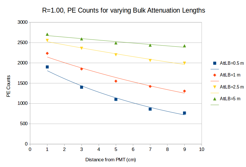
PE Count curves for R=1.00 constant, varying bulk attenuation length
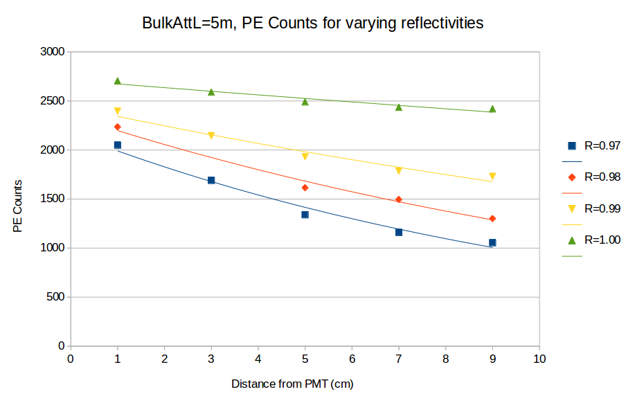
PE Count curves for BulkAttL=5m constant, varying reflectivity
Experimental Raw Data (PTFE)
| DMP-01 (unloaded) | |||||
|---|---|---|---|---|---|
| Distance | 1 | 3 | 5 | 7 | 9 |
| Mean | 2105 | 1822 | 1692 | 1604 | 1538 |
| Sigma | 294 | 237 | 224 | 190 | 121 |
| Par Error | 17 | 27 | 16 | 11 | 12 |
Effective Attenuation Length: 24.9 +/- 2.1 cm
Comparison between R99/2.5, R99/1.0, Experimental data
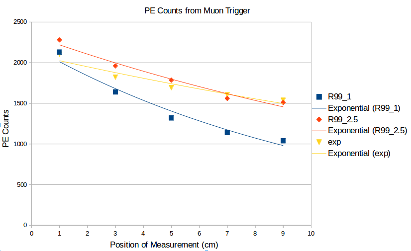
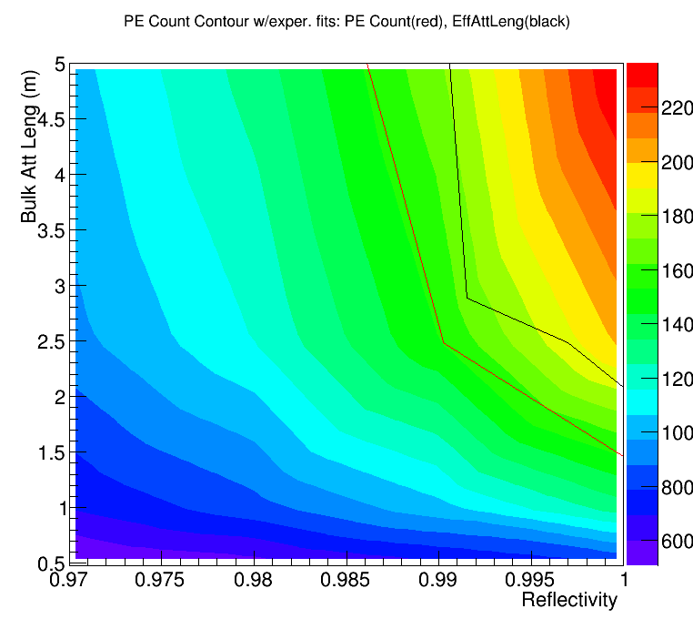
Plotting the experimental data against the computational data, we have the following results:
Effective Attenuation Length contour
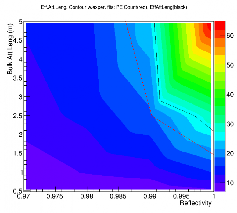
Light output contour