Table of Contents
December 6, before any significant activation
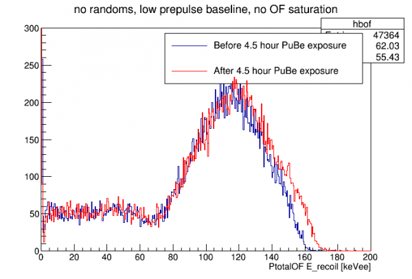
On December 6 we took background data before and after a 4.5-hour exposure to PuBe.
Using pulse integrals I made a partial calibration based on dP/dI information and previously measured phonon collection efficiency.
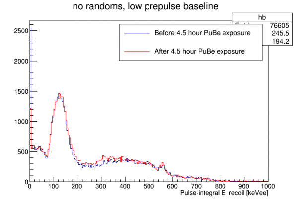 |
| hint of a 511 keV line, maybe |
I calibrated PTOF to the pulse-integral calibration. Note: in this processing I used analytical templates and default (flat) relative calibration so it is not ideal.
 |
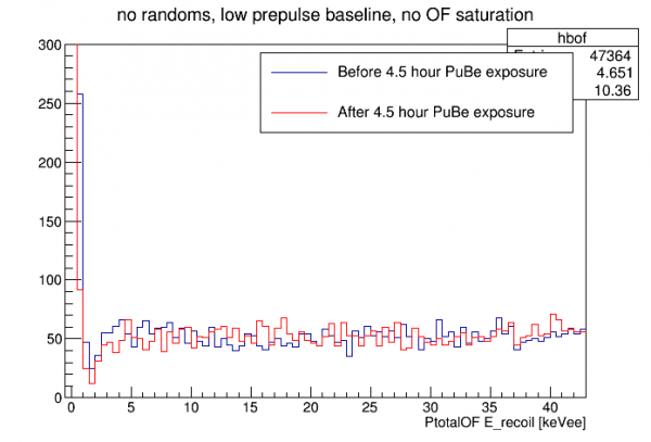 |
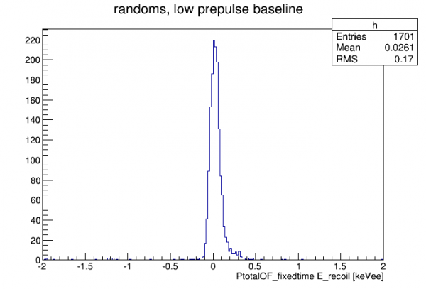
I used the calibration to make a randoms peak to get an idea of the energy threshold:
December 11, after strong activation
On December 6-11 we activated the detector with the PuBe source in its paraffin drum behind the lead shield (weak activation). This produced a significant 10keV line. On December 11 and 12 we performed 2-hour activations with the PuBe source lowered inside the cryostat shield. This made the 10keV line very strong.
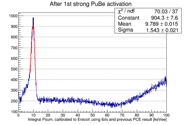
The plot above shows the line using my default calibration based on IbIs-derived dP/dI values and on the phonon collection efficiency I calculated for HV#2 in Run 61. The actual calibration is pretty close, only 6% off! With the line present we can now do accurate calibrations.
Low-threshold data
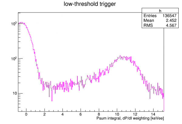
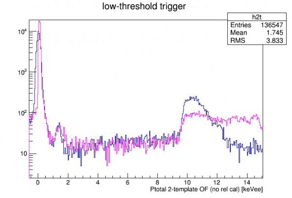
On December 12 we took some data with a low trigger threshold on DCRC1pA (Side1pE, an inner-ring sector channel), in order to try to see the L and M shell peaks. In the integral quantity only the K-shell peak is visible:
Nick processed the data with a 2-template OF fit. (The single template PTOF produces a weird plateau-shaped 10keV line.) The figure below shows the two template amplitudes plotted versus one another:
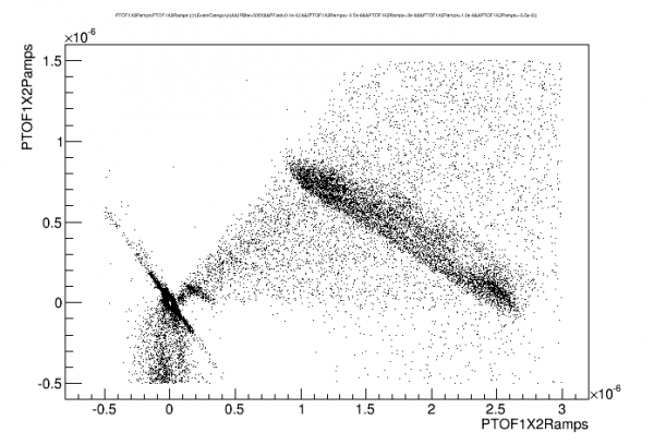
The 10 keV and 1 keV lines are visible as diagonal lines. Fitting the slope we get a linear combination of the two quantities to produce an energy quantity, which is then calibrated:
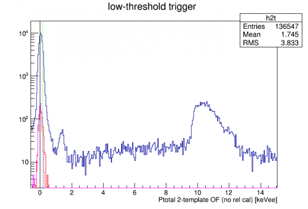 |
| Green line: position of M-shell line Red curve: randoms noise peak, variable t0 Magenta curve: randoms noise peak, fixed t0 |
It should be emphasized that no relative calibration between channels has been applied. Hopefully the peak shapes will improve after we apply this.
Also note: this data (2 hours total) was started 4 hours after ramping up the HV after a flash.
| Comparison of 1-template and 2-template Ptotal OF |
|---|
 |
Relative Calibration
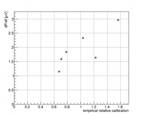
Using December 12 low-threshold data I calculated relative calibrations between the channels. I assume all channels should have on average 1/6 of total energy. Using integrals I plotted the partition of each channel for events in the 10keV region. There is some dependence on energy so it makes sense to choose a low-energy region of interest. Also 10keV should be high enough to avoid any position bias based on the triggering channel. The table below gives the resulting values:
| Relative Calibrations | |
|---|---|
| PA | 1.03746 |
| PB | 0.675776 |
| PC | 1.22766 |
| PD | 0.783613 |
| PE | 1.56723 |
| PF | 0.708266 |
These calibrations have been applied to the automatically processed data in /data/chocula/mast/myProcessedData/midasrq/byseries/ starting on 14 Dec.
If the equal-partition assumption is true, and if the channels have the same phonon collection efficiency, the relative calibrations should scale with the calculated dP/dI values. The plot below compares these and demonstrates an approximate correlation.
Now we need to reprocess recent data with the new relative calibrations. Before doing that we can see what the spectrum looks like with a Psum quantity that adds the individual OF amplitudes with the proper weighting:
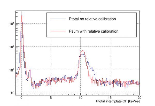
The 10 keV line looks much better. The 1 keV line is not at quite the right place (1.30 keV) - it was closer before the correction. So there may be some non-linearity in the true calibration. The noise peak looks shifted forward, too.