Table of Contents
Run 37
The K100 dilution refrigerator was taken out of service for a few months while maintenance was performed. A number of tasks were performed during this period, including an attempted repair on the tower thermometer wiring at 30 mK and cleaning the PKR 251 pressure sensor attached to the IVC. Problems with the DCRCs were identified at the end of Run 36, and these boards were sent back to Fermilab for repair/upgrade. Additionally, a leak was found in the shaft seal of the He-3 pump, and after an attempted repair, it was sent back to Leybold and a replacement was acquired. A new oil mist eliminator was also placed on the exhaust of the He-3 pump.
A major part of the upgrade was the installation of stripline 27 as a replacement for the broken stripline 21. An additional stripline based on MIT's design was also installed. After completing the upgrade and performing further tests, three broken traces were found on stripline 27. Although two of these traces are QET Return lines that we can live without, Feedback Coil C is also severed. As a result, new PCBs were designed to combine two striplines into one.
Following the aforementioned upgrade, G101b was installed in the fridge with Pb-210 and Am-241 sources in a similar fashion to that in Run 36. The only difference was the removal of the copper shielding covering half the surface of the Pb-210 source.
A base temperature of 70 mK was achieved during this run. As G101b only possesses ionisation channels, Feedback Coil C was not required for this run. Therefore, stripline 27 was connected to side coax ZB1-1-6 and DIB 1 to determine if any further traces have been severed.
The purpose of this run is to investigate the identification of surface events induced by the Pb-210 beta source through a charge symmetry cut. G101b possesses spiral masks consisting of interleaved charge electrodes and grounded rails on both faces of the crystal. The detector features two charge channels on each side: Qi; and Qo. In addition, charge collection efficiency as a function of electric field strength close to the surface is investigated with 60 keV gamma-rays from the Am-241 source.
| Table 1: Run 37 setup | ||
|---|---|---|
| Detector | G101b | |
| Tower | T1 | |
| DIB | 1 | 2 |
| Face | 2 | 5 |
| Side coax | ZB1-1-6 | ZB1-1-9 |
| SQUET | ZC23 | |
| Stripline | 27 | 19 |
| Readout | DCRCv3 | |
-/+ 4 V Pb, Am Data
Am-241 and Pb-210 internal sources
* DIB1 -4 V, DIB2 +4 V
* 0.4096 ms trace length
* 100 us delay
* OR trigger on Qi channels only
* DIB 1 trigger at 32 ADC bins, DIB 2 trigger at 28 ADC bins
* 20/0.1/20 minutes acquisition/flash/cool-down cycle.
* TOTAL EXPOSURE TIME: 440 minutes.
* Collecting electrons on Side 2, Source Side.
* Collecting holes on Side 1, Opposite Source Side.
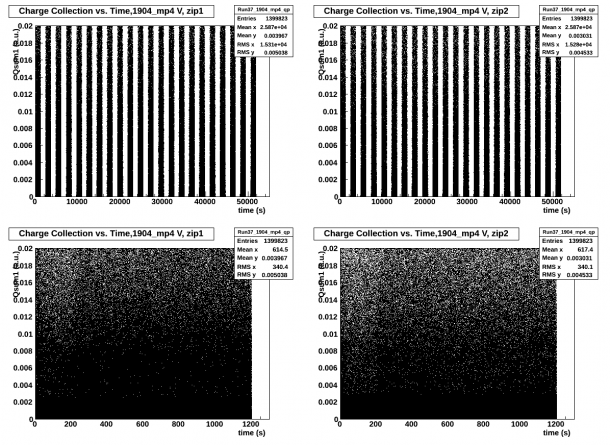
In order to ensure that we were using all of the series and that data was collected for the full 20 minutes, we first created Charge vs Time plots where all of the series were plotted as a function of Δt from the first event collected which can be seen in the top panels of figure 1.1 below for side 1 and side 2, respectively. The bottom panels represent the superimposed collected data of all the data series collected for side 1 and side 2, respectively.
| Fig. 1.1: Charge vs Time, No Cuts, both sides |
|---|
 |
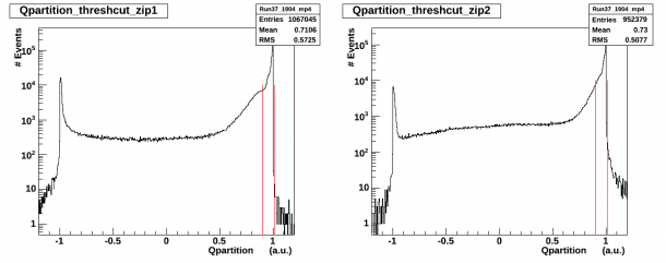
Low energy cuts, were then implemented, Q_sum < 0.00025 (a.u.) where Q_sum = Q_i + Q_o for each side. Low energy cuts will be referred to as thresh_cuts. In order to isolate Q_o dominant events we defined Q_partition = (Q_i - Q_o)/(Q_o + Q_i) and selected only the events which met the 0.9 < Q_partition < 1.01 criteria. The Q_partition distribution after the low energy cuts, thresh_cuts, is displayed in histogram form below in figure 1.2. The red lines identify the 0.9 < Q_partition < 1.01 cut.
| Fig. 1.2: Q_partition distribution, thresh_cuts, both sides |
|---|
 |
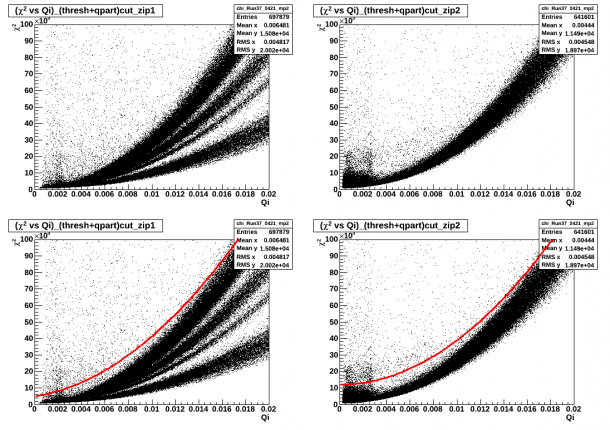
The quality of the pulses was then checked by plotting q_i vs. chi_square for all events which passed the thresh and Q_partition cuts. A second order polynomial was fit to the distribution and was used to implement the final chi_square cut which is then plotted in red in the bottom panels of figure 1.3. The Q_i 2 vs. chi_square plot, on the right side of figure 1.3, top and bottom, exhibited a large concentration of low energy events.
| Fig. 1.3: Qi vs Chi_square, thresh and Q_partition cuts, both sides |
|---|
 |
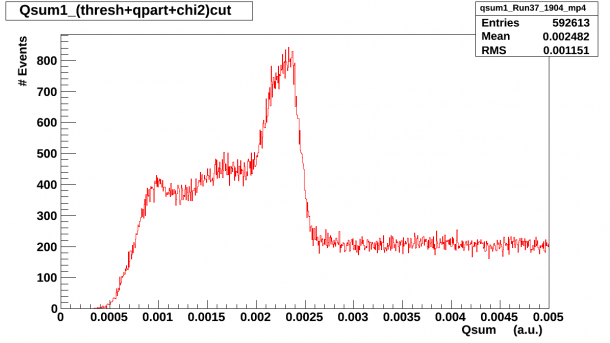
Finally, we plotted the spectra, in a.u. units for both sides where only respective individual side quality cuts were implemented. The top panel of figure 1.4 is the side 1 spectra, opposite source side and the bottom panel of figure 1.4 is the side 2 spectra, source side.
| Fig. 1.4: Qsum a.u. spectra, thresh + Q_partition + chi_square cuts, both sides |
|---|
 |
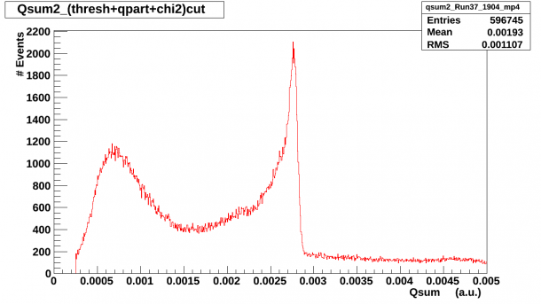 |
The Am-241 peak is visible on side 2 as well as a low energy hump in the [0.0005, 0.001] a.u. range which roughly corresponds to a [12, 22] keV range by calibrating to the 60 keV peak at 2.89124e-04 a.u. The Am-241 peak is also visible on side 1. A Ba-133 exposure data set was used to calibrate the keV range but only side 2 presented a visible peak which could be calibrated. Fig. 1.5 below shows the calibrated keV spectra for side2.
| Fig. 1.5: Qsum2 spectra, keV |
|---|
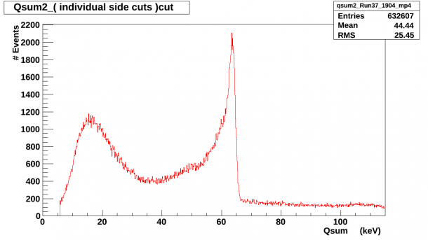 |
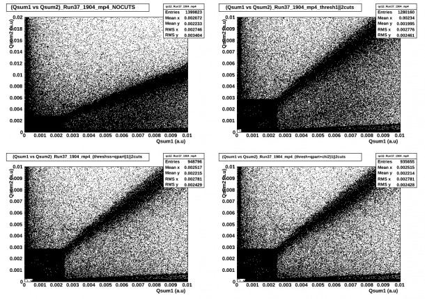
Figure 1.6 below shows the Qsum1 vs. Qsum2 spectra as the individual cuts are implemented sequentially and OR'ed.
| Fig. 1.6: Qsum1 vs. Qsum2 spectra |
|---|
 |
In order to identify side 2 surface events we have:
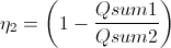
thus, we can define surface events on side 2 as Q_sum2 dominated events for which .9 < η2 < 1.01.
Similarly, in order to identify side 1 surface events we have:
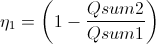
where we can define surface events on side 1 as Q_sum1 dominated events for which .9 < η1 < 1.01
Bulk events can be identified by looking at those events for which neither Q_sum1 or Q_sum2 is dominant
- etta1_cut_bulk = -0.4 < η1 < 0.4
- etta2_cut_bulk = -0.4 < η2 < 0.4
and
- bulk_cut = etta2_cut_bulk||etta1_cut_bulk
Side 2 Surface Events
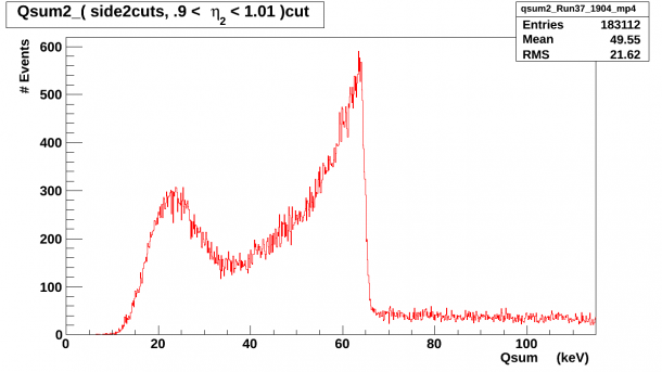
Figure 2.1 below shows the side 2 keV spectra after the .9 < η2 < 1.01 cut has been added to the individual side2 quality cuts.
| Fig. 2.1: Qsum2 keV spectra with side2cuts and η2 surface events cut. |
|---|
 |
In order to investigate what these events looked like on side 1, the same cuts were implemented on the Qsum1 spectra i.e. side2cuts and .9 < η2 < 1.01 cut and the results can be seen below in Figure 2.2.
| Fig. 2.2: Qsum1 a.u. spectra with side2cuts and η2 surface events cut. |
|---|
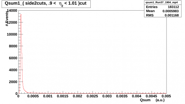 |
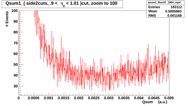
There is a large dominance of low energy events and in order to ensure that no feature existed in the expected Am-241 region the y-axis scale was reduced to 100 and the result can be seen below in Figure 2.3.
| Fig. 2.3: Qsum1 a.u. spectra with side2cuts and η2 surface events cut, zoom to 100. |
|---|
 |
As a final check that no surface events on side 2 create a spectral feature on side 1, the .9 < η2 < 1.01 cut was implemented with the side1cuts on the Qsum1 spectra and the results can be seen below in Figure 2.4.
| Fig. 2.4: Qsum1 a.u. spectra with side1cuts and η2 surface events cut. |
|---|
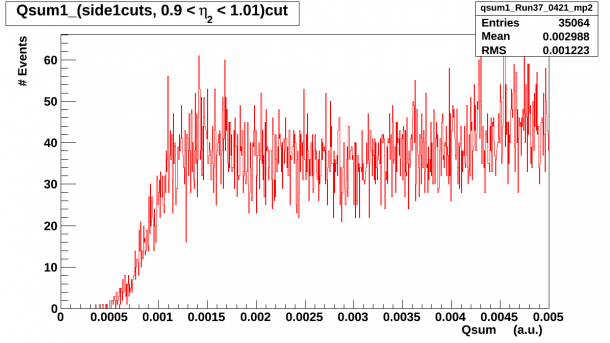 |
In conclusion, side 2 surface events which are defined as
approaches unity, .9 < η2 < 1.01, do not correspond to those events which create the 60 keV feature on side1.
A further investigation was undertaken to investigate the surface events spectra at higher energy as observed on side 2. Figure 2.5 below shows the Qsum2 spectra with side2cuts and .9 < η2 < 1.01 cut as the range was extended beyond 2.5 MeV with the same scaling/binning as in Figure 2.1.
| Fig. 2.5: Qsum2 keV spectra with side2cuts and η2 surface events cut, x-axis extended beyond 2.5 MeV. |
|---|
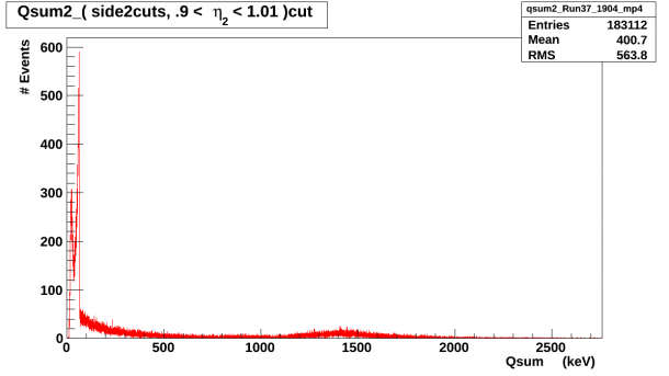 |
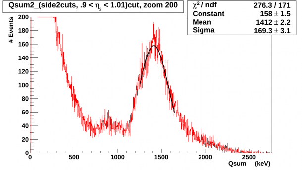
A feature is noticeable around 1.4 MeV and that area of interest was zoomed in and it was Gaussian fitted to identify the mean. The spectrum, fit parameters and the goodness of fit can be seen below in Figure 2.6.
| Fig. 2.6: Qsum2 keV spectra with side2cuts and η2 surface events cut, x-axis extended to 2.5 MeV, zoom to 200. |
|---|
 |
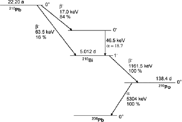
The decay scheme for Pb-210 can be seen below in figure 2.7, taken from L. Laureano-Perez, et al., “A liquid-scintillation-based primary standardization of Pb-210”, Appl. Radiat. Isot. 65 (2007) 1368.
| Fig. 2.7 Pb-210 Decay Scheme |
|---|
 |
| http://www.sciencedirect.com/science/article/pii/S0969804307001960 |
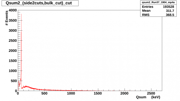
Possible contributions to this feature could come from K-40 in the S34 background or from the quenched 5.3 MeV alpha decay of Po-210. As a check of this, the bulk_cut was introduced and the resulting spectra can be seen below in figures 2.8 and 2.9.
| Fig. 2.8 Qsum2 spectrum, side2cuts&&bulk_cut |
|---|
 |
| Fig. 2.9 Qsum2 spectrum, side2cuts&&bulk_cut, zoom to 200 |
|---|
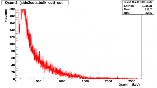 |
No feature is present around 1.4 MeV in figures 2.8 and 2.9 which would eliminate the possibility that the 1.4 MeV features present in figure 2.6 is due to 1.42 MeV gammas resulting from K-40 in the natural background of our laboratory.
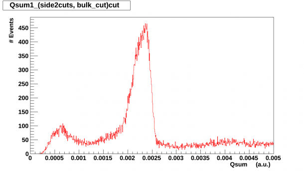
The bulk_cut was then introduced with each individual side cut and the resulting spectra can be seen below in figures 2.10 and 2.11.
| Fig. 2.10 Qsum1 spectrum, side1cuts&&bulk_cut |
|---|
 |
| Fig. 2.11 Qsum2 spectrum, side2cuts&&bulk_cut |
|---|
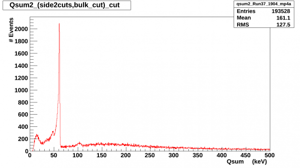 |
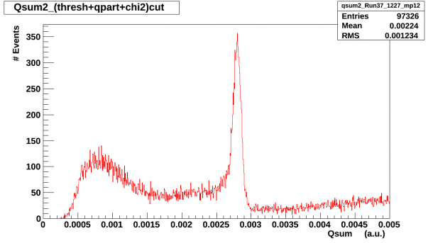
One troubling feature present in figure 2.8 and 2.9 is the low energy bump in the [12,22] keV region. The Am events on side 1 are to be expected as we know that some Am events do penetrate across to side 1 but if the low energy bump on the side 2 spectrum is due to Pb-210 betas then they should not be present on side 1 and they should not be present when looking at bulk events on side 2.
Side 1 surface events
In order to ensure that we are not biasing ourselves by only looking at Qsum2 dominant events as defined by the .9 < η2 < 1.01 criteria, Qsum1 dominant events were also isolated by selecting the data points which meet the .9 < η1 < 1.01 criteria. The resulting spectrum can be seen below in figure 3.1.
| Fig. 3.1: Qsum1 a.u. spectrum with side1cuts and .9 < η1 < 1.01 cut. |
|---|
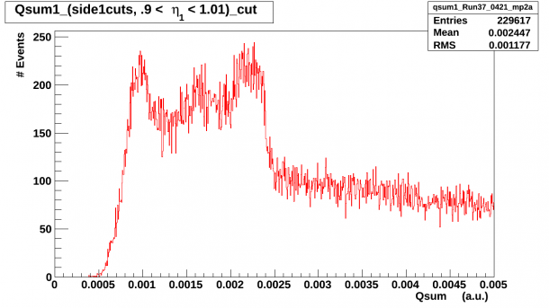 |
No clear explanation was found for the tri-peak feature visible in the Qsum1 spectrum and in order to investigate the events as they look on side2 a Qsum2 spectrum was drawn using the same cuts, side1cuts and .9 < η1 < 1.01 cut. A large dominance of low energy events was present as can be seen below in figure 3.2.
| Fig. 3.2: Qsum2 keV spectrum with side1cuts and .9 < η1 < 1.01 cut. |
|---|
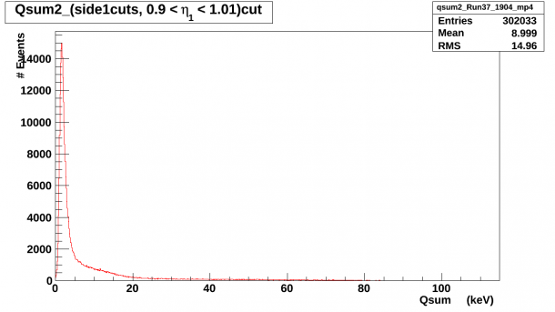 |
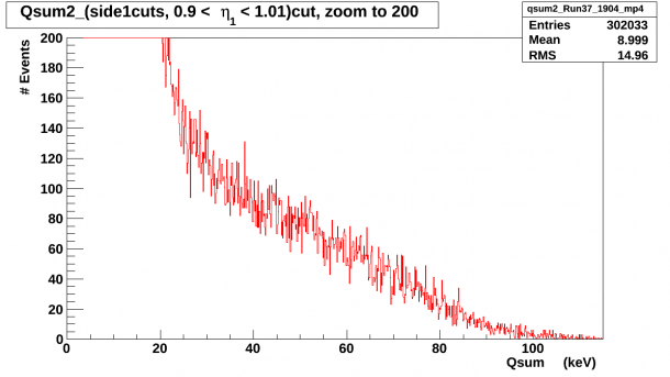
In order to ensure that large low energy peak wasn't overshadowing another feature, we zoomed in to 200 on the y-axis and the resulting spectrum can be seen below in figure 3.3.
| Fig. 3.3: Qsum2 keV spectrum with side1cuts and .9 < η1 < 1.01 cut, y-axis zoom to 200. |
|---|
 |
-/+ 12V Qpartition double peak
A double peak is observed in the Qpartition plot on side 2 at large biases when it collects electrons, + bias. The feature can be seen below in figure 4.1 for the -/+ 12V data. This feature started to develop in the -/+ 8V data set and its' prominence increased in the -/+ 10V set and then became even more pronounced in the -/+ 12V data.
| Fig.4.1 Qpartition plot, -/+ 12V, side 2 |
|---|
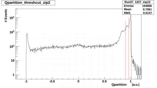 |
The red lines in figure 4.1 above denote the two Qpartition cuts which were implemented in order to investigate the contribution of those events to the Qsum2 spectrum.
The cuts implemented are :
- 0.9 < Qpartition < 0.96
- 0.96 < Qpartition < 1.01
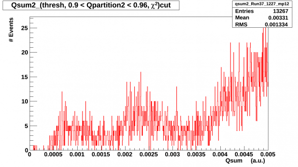
The resulting spectra after implementing the above Qpartition cuts and performing a new χ^2 fit can be seen below in figure 4.2 and figure 4.3. This feature started to develop in the -/+ 8V Qpartition side 2 plot whose prominence increased in the -/+ 10V set and then became even more pronounced in the -/+ 12V data.
| Fig.4.2 Qsum1 plot, -/+ 12V, thresh + chi2 + (0.9 < Qpartition < 0.96) cut |
|---|
 |
| Fig.4.3 Qsum1 plot, -/+ 12V, thresh + chi2 + (0.96 < Qpartition < 1.01) cut |
|---|
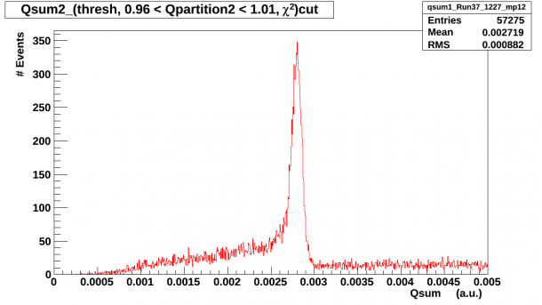 |
It is quite surprising that the low energy hump disappears in figure 4.3. The Pb-210 source does cover part of Qo and we did notice a slight broadening of the +1 peak in the Qpartition spectra but the double peak became visible around -/+ 8V and was only present when collecting electrons on side 2.
The original spectra with its own side quality cuts and 0.9 < Qpartition < 1.01 cut can be seen below in figure 4.4.
| Fig.4.4 Qsum1 plot, -/+ 12V, side2cuts |
|---|
 |
low energy feature at low biases
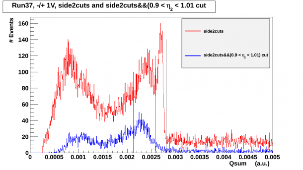
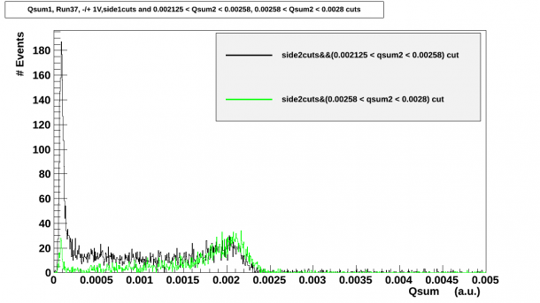
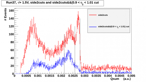
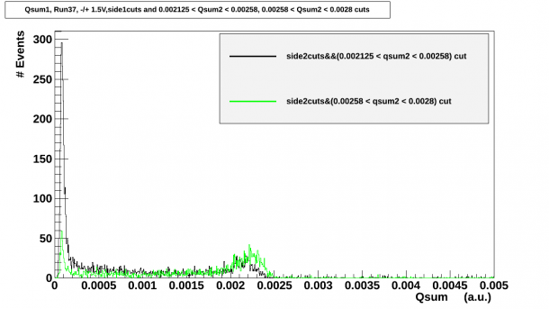
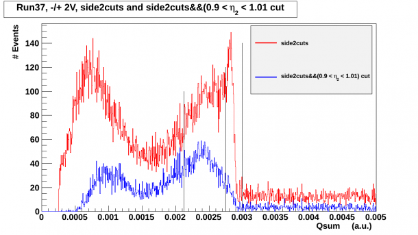
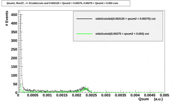
At low biases biases a broad feature was present before the Am_peak when collecting electrons on side 2, source side. This feature was observed at -/+ 1V, -/+1.5V and -/+2V. A η2 surface event cut was then added to each spectra, 0.9 < η2 < 1.01 and the Am peak and broad feature were isolated and those events were selected. The associated Qsum1 collection for the same events was then plotted, as can be seen below. The troubling feature in the figures below is that when implementing 0.9 < η2 < 1.01 the Am peak disappears. This behavior is no longer present by the time we get to -/+ 4V data set as was shown in figure 2.1. For the seagull plots in the following section, it was these peaks which disappear when implementing the 0.9 < η2 < 1.01 cut that were used for the calibration peak.
- -/+ 1V
| Fig.5.1 Qsum2 plot, -/+ 1V |
|---|
 |
| Fig.5.2 Qsum1 plot, -/+ 1V |
|---|
 |
- -/+ 1.5V
| Fig.5.3 Qsum2 plot, -/+ 1.5V |
|---|
 |
| Fig.5.4 Qsum1 plot, -/+ 1.5V |
|---|
 |
- -/+ 2V
| Fig.5.5 Qsum2 plot, -/+ 2V |
|---|
 |
| Fig.5.6 Qsum1 plot, -/+ 2V |
|---|
 |
Seagull Plots
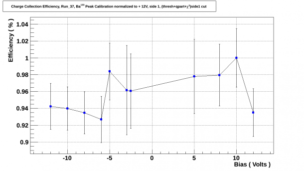
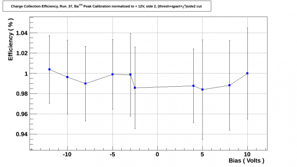
When fitting for the Ba and Am features only individual side cuts were used due to the influence of the η cuts at low biases.
| Fig. 6.1 Ba peak calibration, side 1 |
|---|
 |
| Fig. 6.2 Ba peak calibration, side 2 |
|---|
 |
| Fig. 6.3 Am peak calibration, side 2 |
|---|
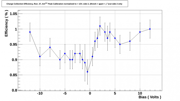 |
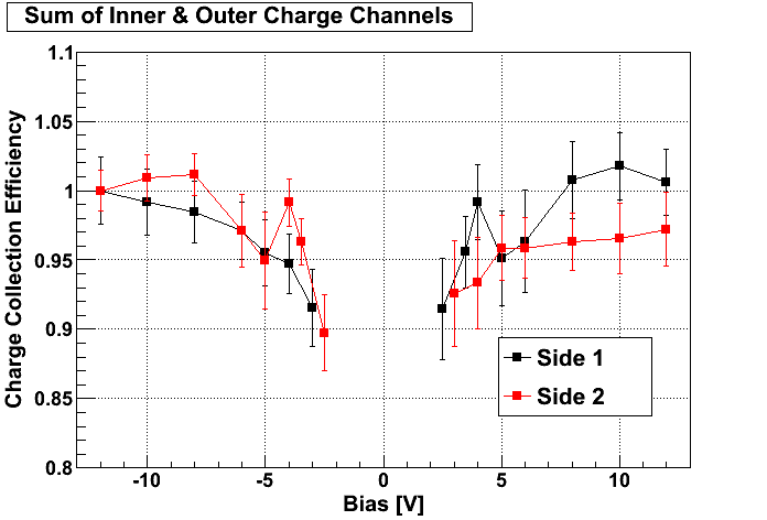
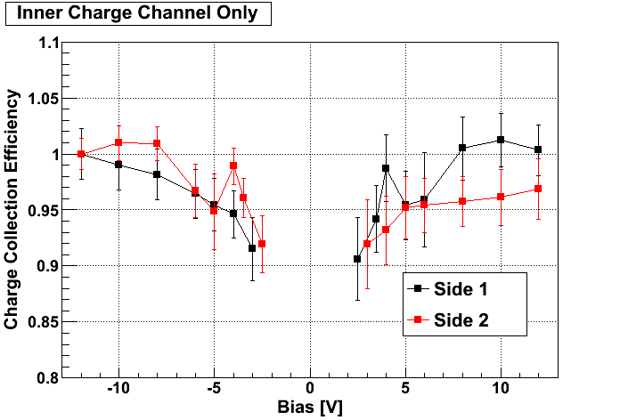
For comparison, the seagull plots for Run 28 can be seen below in figures 6.4 and 6.5. When looking at side 2 in figure 6.3, we can see that charge collection efficiency, when collecting holes on side 2 at low biases, dips down to 86%, well below the charge collection efficiency observed in Run 28. Also, when looking at figure 6.1 we can see that charge collection efficiency takes a sudden drop when collecting electrons as we increased the bias to -/+ 12V from -/+10V. It is important to note that the Run 28 data was collected without the shield which would have had an impact on the Ba-peak.
| Fig. 6.4 G101b, Run 28 Charge Channel Efficiency, Oi |
|---|
| Fig. 6.5 G101b, Run 28 Charge Channel Efficiency, Osum |
|---|