Table of Contents
Run 32 : G103a (100 mm iZIP) Test - Round 2
Summary
Summary presented at DTC meeting on Monday 19th December 2012.
In this run we have reached a base temperature of 59 mK, and it is the same detector configuration (as with striplines and SQUET cards as well) as Run 31.
Charge Studies
Charge Signal Baseline
| Figure 1 - 0 V bias |
|---|
| 07121020_2016 |
| Left: Zip 1; Right: Zip 2 |
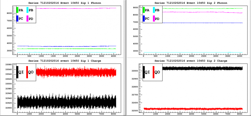 |
| A glimpse of the charge and phonon pulses' baseline during the first 500 events. This is event #464. |
Charge Spectra and Stability
In Run 31 several data sets were taken where triggering happened solely on the charge channels or the phonon channels. We wanted to look into the data to see what effect this had on the spectra. Figures 2 and 3 are at the same bias and trigger settings (on charge channels only) but with reversed polarity. Figure 4 shows data at the same bias and with the same polarity as Figure 2's data. However, Figure 4 shows the spectra for phonon channel triggering. Unfortunately, we discovered later on after taking the data that the detector was not flashed properly before the data shown in Figure 4. We do see some interesting features, still, which is why we felt it worth mentioning below.
| Figure 2 - Dib1: +4 V, Dib2: -4V | |
|---|---|
| Trigger on *charge* channels | |
| 07120807_1306, 07120807_1356, 07120807_1447 ; 30 min/series | |
| (Qi/DIB1, Qo/DIB1, Qi/DIB2, Qo/DIB2) at (56, 40, 32, 32) ADC bins | |
| First 15 minutes | Full run |
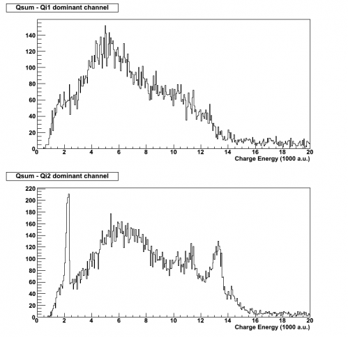 | 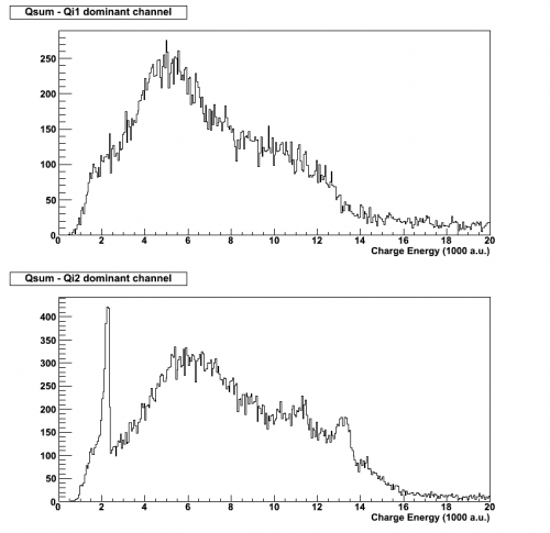 |
| Triggering on the charge channels only provides a distinct 60 keV peak from the Am-241 source on side 2 and we also see evidence for the 356 keV peak from the Ba-133 source on the same side. | |
| Figure 3 - Dib1: -4 V, Dib2: +4V | |
|---|---|
| Trigger on *charge* channels | |
| 07120806_2157, 07120806_2247, 07120806_2337 ; 30 min/series | |
| (Qi/DIB1, Qo/DIB1, Qi/DIB2, Qo/DIB2) at (56, 40, 32, 32) ADC bins | |
| First 15 minutes | Full run |
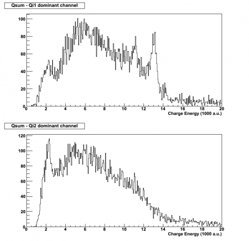 | 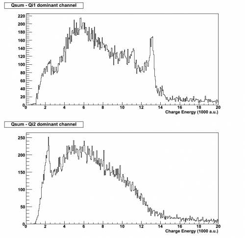 |
| Flipping the polarities, and with all other settings kept the same, we still see the 60 keV peak on side 2 (which is to be expected), and the 356 keV peak is on side 1 now. This indicates that the 356 keV peak appears predominantly on the side that collects holes. | |
| Figure 4 - Dib1: +4 V, Dib2: -4V | |
|---|---|
| Trigger on *phonon* channels | |
| 07120728_0959 ; 2 hours | |
| Phonon trigger: 20 ADC bins | |
| First 15 minutes | Full run |
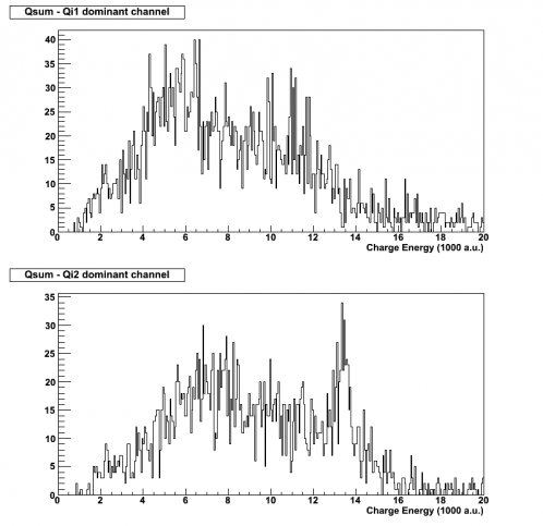 | 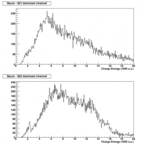 |
For Figure 4's data set, there was no flashing beforehand (incorrect LED bias). However, the detector was grounded for 20 minutes, which might be a reason for the presence of the 356 keV peak in the first 15 minutes. After the full 2 hours, this peak disappears due to poor neutralization but then we do see a small signature of the 60 keV peak that wasn't present in the first 15 minutes. There is some suspicion that triggering only on the phonon channels does not effectively show us the 60 keV peak as triggering on the charge channels do. Looking back to Figure 2's first 15 minutes, there was a clear signature of both peaks. In Figure 4's first 15 minutes, there is only a small 356 keV peak. Despite the low statistics, seeing no hint of the 60 keV peak is interesting.
It may also be worth to note that the data taken previously to Figure 4's was +/- 2 V, which might be a reason for the somewhat visible 356 peak in the first 15 minutes of this -/+ 4 V set.
The reason for the low statistics may be due to the trigger selection or the flashing- this will have to be investigated. Further studies will be made into charge vs. phonon triggering (with proper prior flashing, of course) to determine if the behavior we're seeing in the data persists. It will also be good to study further whether or not flipping polarities (with all other settings and conditions constant) has an effect on charge stability and collection. Figure 3 suggests that with Side 2 positively biased, collection is less effective.
Charge Collection Efficiency
| Figure 5 : Ba-133 Peaks from Run 31 |
|---|
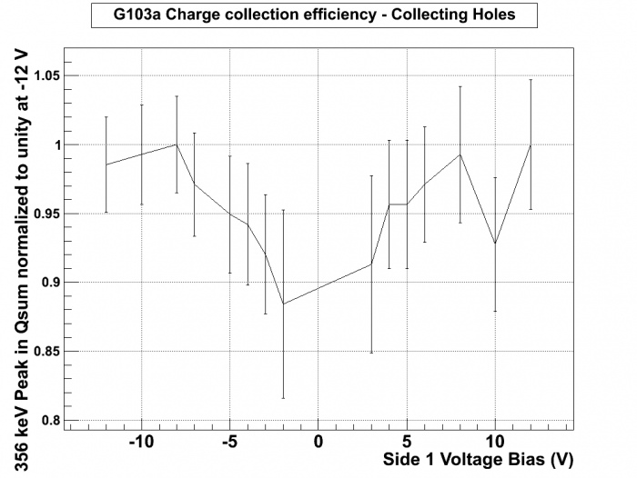 |
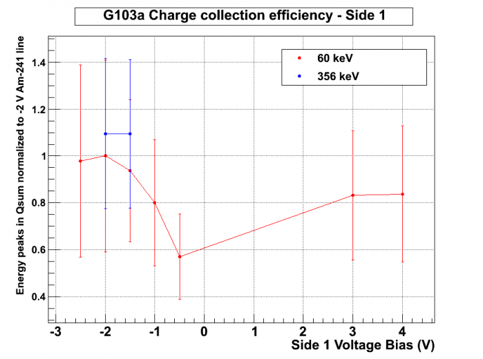
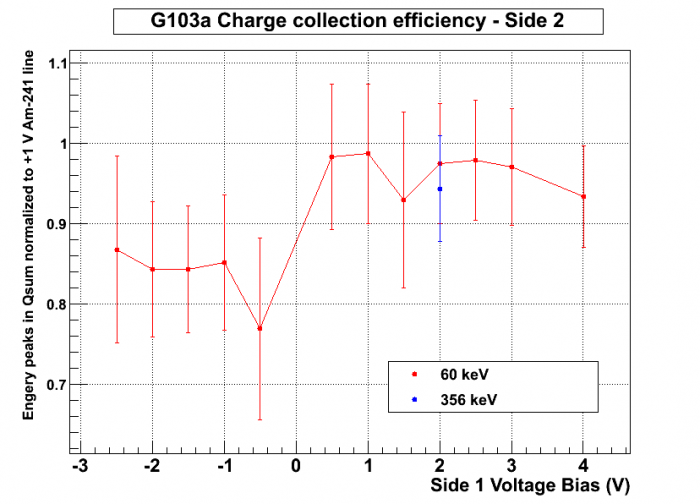
This is a preliminary examination of the charge collection efficiency for G103a based on Run 31's data. No data with suspected poor flashing was used. The peak selected for this charge collection efficiency study was the 356 keV peak from the external Ba-133 source, and points were only selected from the side collecting holes. The voltage biases are written based off of Side 1's bias.Peaks were not detected in the lower biases of +/-2 V, +/-1 V, and -/+ 1 V. We can try to retake data with these biases in this run to detect a peak.
Below are charge collection efficiency plots from Run 32 data. This is a study into the collection efficiency of each side of G103a. We are currently lacking points for 356 keV peaks at low biases, but the few points we have are plotted on the same plots as values obtained from 60 keV peaks. Each side is calibrated to a specific peak value, denoted by the y-axis. Both 60 keV and 356 keV peaks are calibrated to the same peak (assuming a linear energy scale for the 356 keV peak).
| Figure 6 & 7 : Peaks from Run 32 |
|---|
 |
 |
Phonon Studies
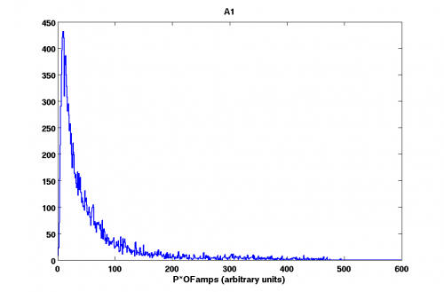
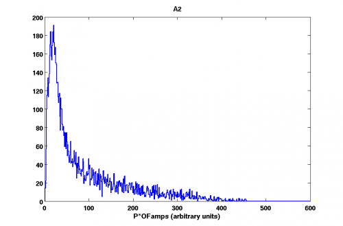
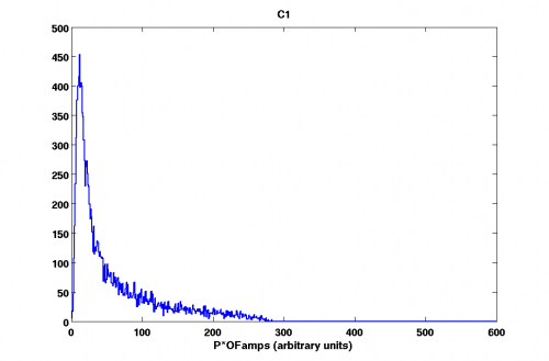
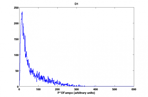
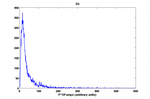
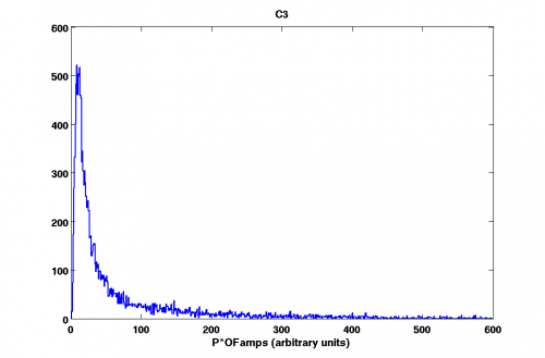
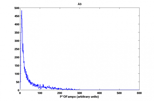
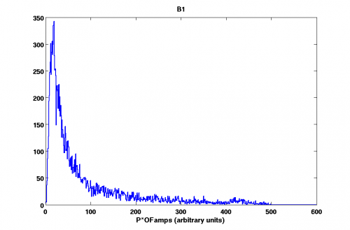
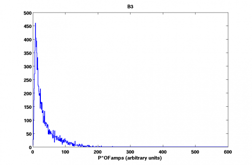
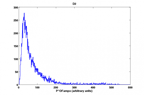
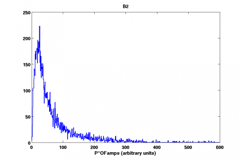
Histograms of phonon energies (P*OFamps) (07121012_0136).
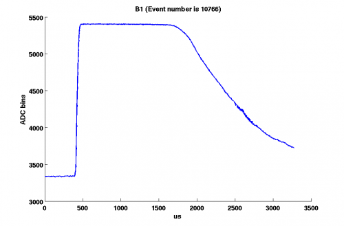
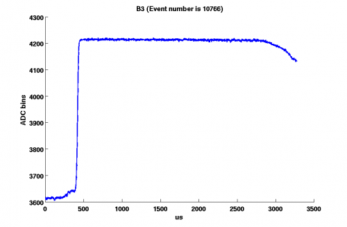
One can notice that maximum energy deposited to the phonon channels on the side 1 is ∼ 2 times as greater as that for side 2.
Notice that energy is measured in arbitrary units (it's RQ value). It was not possible to make a calibration for the phonon channels.
| Fig. 6. Four inner channels | |
| Side 1 | Side 2 |
|---|---|
 |  |
 |  |
 |
|
 |  |
| Fig. 7. Central channels | |
| Side 1 | Side 2 |
 |  |
| Fig. 8. Outer channels | |
| Side 1 | Side 2 |
 |  |
| Fig. 9. Four inner channels | |
| Side 1 | Side 2 |
|---|---|
 |  |
 | 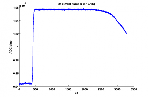 |
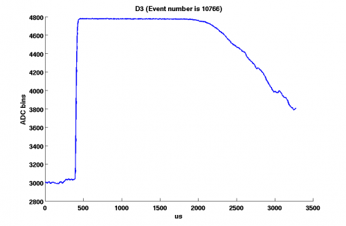 |
|
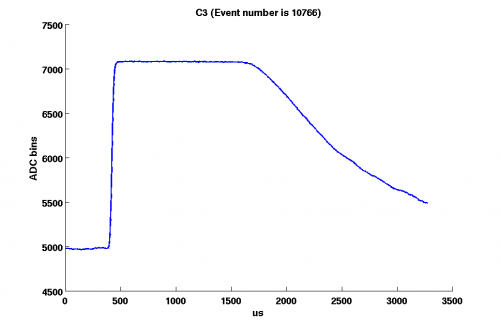 | 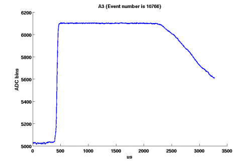 |
| Fig. 10. Central channels | |
| Side 1 | Side 2 |
 |  |
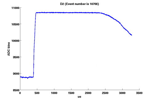
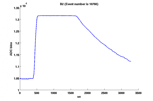
| Fig. 11. Outer channels | |
| Side 1 | Side 2 |
 |  |
Identical pulses
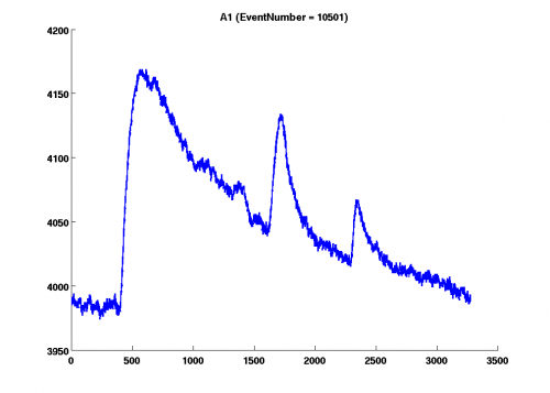
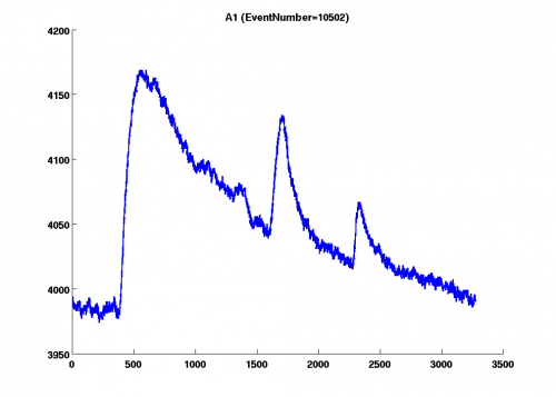
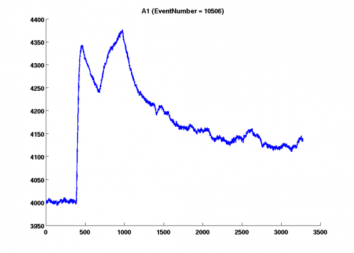
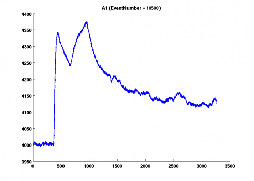
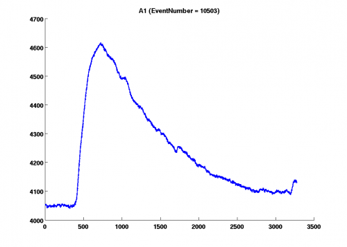
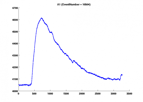
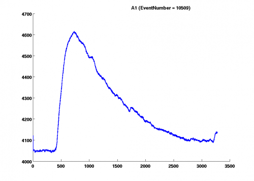
Identical pulses (X = time in ms) (Y = number of bins) (07121012_0658). This is an issue we have encountered. As one can see in most cases identical pulses occur in successive events. However sometimes this is not the case.
 |  |
|---|---|
 |  |
Phonon Pulses Decay Time
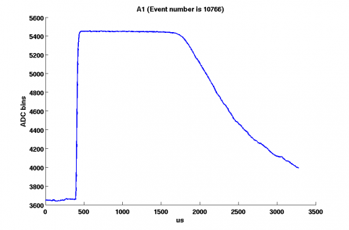
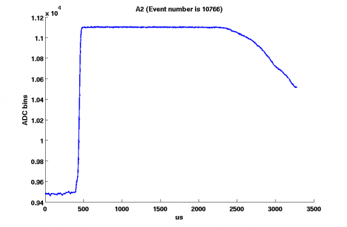
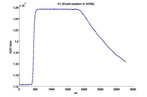
I consider data series 07121014_0839. Select only good events, the ones that survive the cuts applied.
The cuts are:
1) Chi^2 for charge(RQ value)
2) Low energy cut (charge as well)
4) Positive phonon energy.
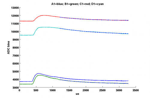
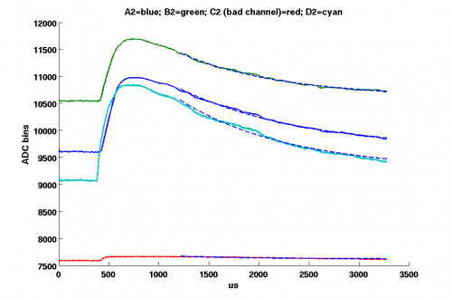
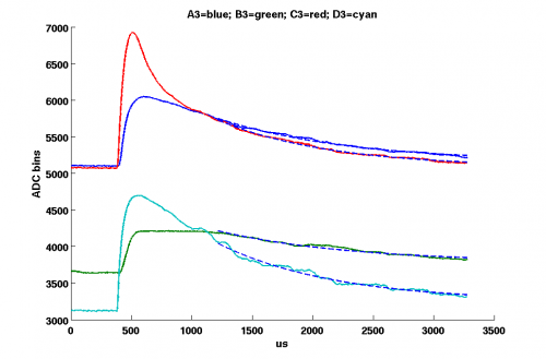
The next step is to fit the selected phonon pulses with the function F=A*Exp(-t/T_decay)+B, where B is the offset.
I fit the pulses starting from 800 (us) from the point where the pulses start to rise. The quantity of interest is the T_decay. It turns out that the decay time constant is the same (within the error) for all channels.
In fig.1 one can see an example of the fit.
| Fig. 1. Example of the fit. | ||
|---|---|---|
 |  |  |
The values of the decay time constant are:
| zip1 | zip2 | zip3 |
|---|---|---|
| A1→ 841 ± 166 (us) | A2→ 970 ± 230 (us) | A3→ 902 ± 162 (us) |
| B1→ 853 ± 164 (us) | B2→ 905 ± 174 (us) | B3→ 916 ± 195 (us) |
| C1→ 866 ± 144 (us) | C3→ 876 ± 165 (us) | |
| D1→ 937 ± 197 (us) | D2→ 1060 ± 261 (us) | D3→ 961 ± 218 (us) |