| DIB1pA IbIs curve [V versus μA] |
|---|
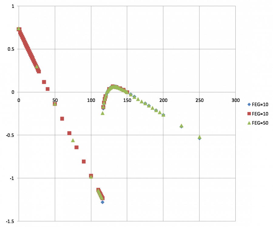 |
| The three series were taken with different driver offsets. In this plot they have been shifted so that a common bias (150 μA) is at zero. It's noteworthy and very useful that there are no SQUID phase jumps from 0 μA all the way up to transition. |
| DIB1pA IbIs zoom on transition region [V versus μA] |
|---|
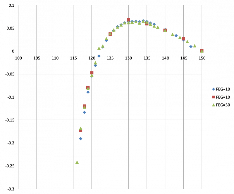 |
| The series are in rough agreement but there are definitely shifts in Vout. |
| DIB1pA IbIs slope [V/μA versus μA] |
|---|
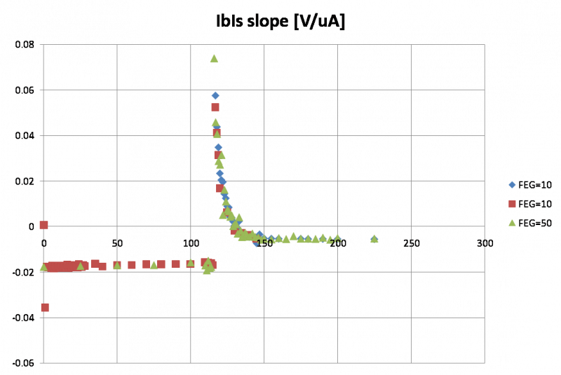 |
| This is the point-to-point slope of the IbIs curve. |
| DIB1pA IbIs slope zoom on superconducting region [V/μA versus μA] |
|---|
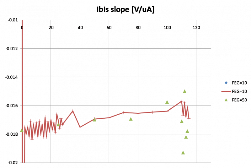 |
| The slope does not stay constant throughout the s/c region, and increasing the front-end gain from 10 to 50 doesn't help much. The zig-zag seen in the points taken in 1-μA increments makes me wonder if there is an ADC rounding artifact when QET biases are entered to the nearest μA. |
| DIB1pA IbIs slope zoom on superconducting region [V/μA versus μA] with corrected QETbias |
|---|
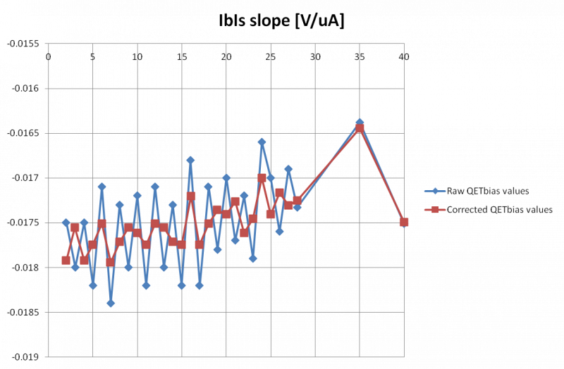 |
| It turns out that the zig-zag is indeed caused by QET bias rounding. The QETbias setting ranges -1600 to 1600 μA with a 16-bit resolution. That comes to 20.48 ADC bits per μA. So after rounding the actual division between 1 μA steps will alternate between 20 and 21 ADC bits. There are 0.048828125 μA per ADC bit so the rounding error can be as high as about ± 0.025 μA. The plot shows the effect of correcting the QETbias for the rounding error. The scatter is smaller and appears random after the correction. |
| DIB1pA IbIs slope zoom on normal region [V/μA versus μA] |
|---|
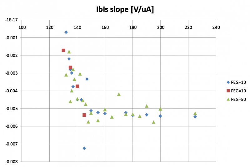 |
| This plot suggests a nearly linear region between 160 and 240 μA. No noticeable improvement with front-end gain of 50. |
| DIB1pA IbIs with offset fits [V versus μA] |
|---|
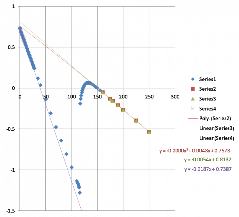 |
| Here the two front-end-gain=10 series were used. Three offset estimates are shown: 1) linear fit to normal region 2) quadratic fit to normal region 3) linear fit to s/c region near zero Although the normal region appears linear there is a distinct difference between linear and quadratic offset estimates. The quadratic estimate is close to the (presumably correct) fit to the s/c region, but there is still a 20 mV discrepancy. Both the s/c and normal parts of the IbIs are slightly curved, but the curvatures are in the opposite direction. If the curvature is due to an error signal in the SQUID amplifier circuit it probably wouldn't explain why these are opposite. And the fact that changing the front-end gain from 10 to 50 doesn't change either curvature also suggests that it's not due to an error signal. |
| DIB1pA Rtes+Rpar versus Ib [mΩ versus μA] |
|---|
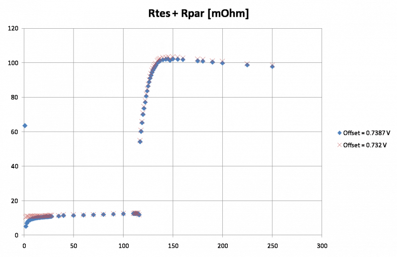 |
| Resistance versus Ibias calculated based on absolute Is with standard assumptions. Another slight shift in offset by 9 mV seems to make the superconducting region more uniform. |
| DIB1pA Ptes versus Ib [pW versus μA] |
|---|
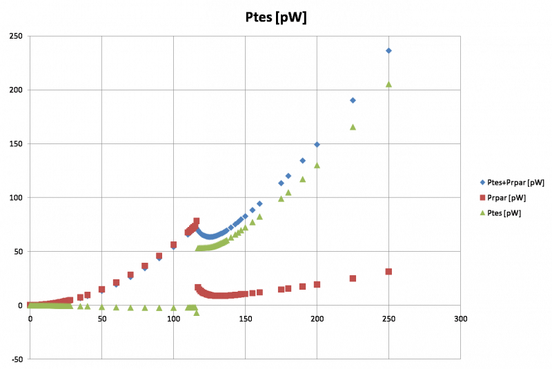 |
| Power dissipated in TES by Is versus Ib. The total power in the TES branch, TES + parasitic, can be calculated from just Ib and Is (and Rshunt). To calculate the power in the parasitic resistance I assume that Rparasitic = 13 mΩ (this is an average value over the full s/c range if Rpar is calculated from dIb/dIs rather than absolute Ib/Is). Subracting gives the TES power |
| DIB1pA Ptes versus Ib zoomed to transition region [pW versus μA] |
|---|
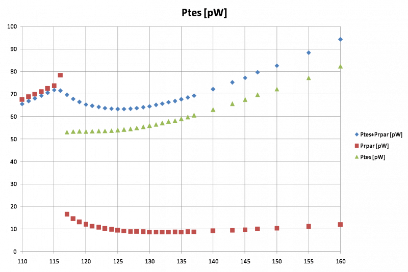 |
| The TES equilibrium power in transition is roughly constant, rising slowly as would be expected from a finite width in transition temperature. It starts at around 53 pW at the bottom of the transition, rising to about 54 pW at 125 μA closer to the top of the transition, then faster to about 56 pW near the IbIs peak. After that it transitions into the quadratic shape expected in the normal part. |
| DIB1pA Rpar versus Is [mΩ versus μA] |
|---|
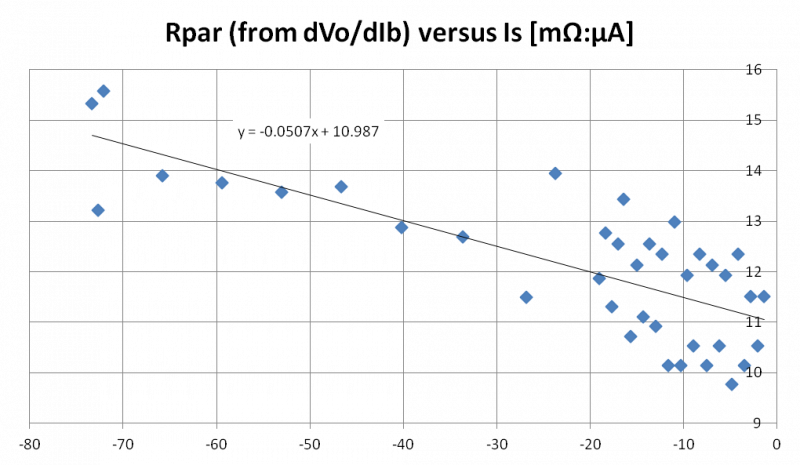 |
| Parasitic resistance versus Is (the current through the TES) calculated based on IbIs slope. If the dependence of Rpar on Ibias seen above is not an artifact of the SQUID circuit (which the insensitivity to front-end gain suggests) then perhaps it is physical. This plot would then indicate the parasitic resistance increases with current through the TES. This is relevant in the prefactor calculation. The slope of the IbIs curve in the superconducting region is an element in the calculation, but it is not constant. The correct value to use would be one taken at the same Is as the operating point. As can be seen in the first plot on this page, the correct slope should be one measured at an Ibias of around 50 μA. |
| DIB1pA Prefactor versus Ibias [μA] |
|---|
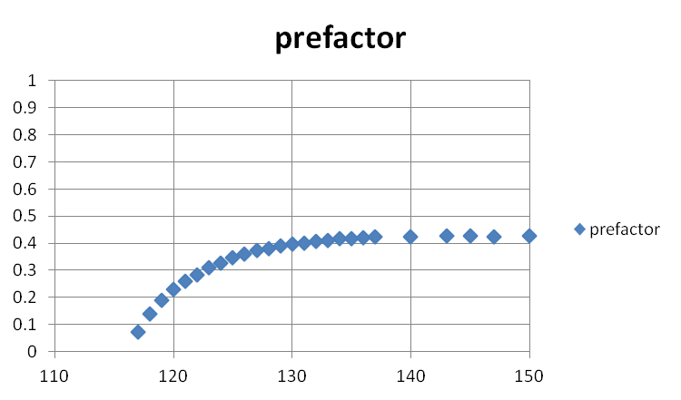 |
| Here the dP/dI prefactor is calculated. The dVo/dIb-at-s/c value used was -0.017 V/μA, taken from the plot above. The uncertainty is perhaps 0.0002, which shifts the lower prefactor values significantly. |
| DIB1pA Prefactor*Ibias versus Ibias [μA] |
|---|
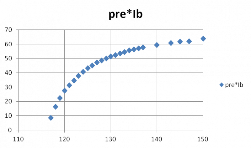 |
| Here the product of prefactor and Ibias is shown. This product gives the relative dP/dI value. From this plot it looks like we could choose values of 10, 20, or 40. Assuming the channel can be calibrated, comparing data at these three settings should provide a chance to verify the dP/dI calculation. |