Origin of the sharp peaks in the average noise PSD; the 408 kHz line

Note 7 · Author(s): Anthony Villano · 23 Sept 2026 (revised 22 Oct 2026) · Status: In progress

Caution (2026-10-22): the sample time has changed. The phonon sample period is 0.8 µs (1.25 MHz), not the 1.6 µs (625 kHz) this note was written with (see The sample period in python/README.md for the evidence). What changed in this note:

Every frequency in this note is twice the value the first version gave: the line called “the 204 kHz line” is at 408 kHz (408,020 Hz), and the seven flagged lines are at 52.8, 84.5, 155.3, 211.2, 366.5, 372.9 and 408.0 kHz (not 26.4, 42.3, 77.7, 105.6, 183.3, 186.5 and 204.0 kHz). The lowest bin is 305 Hz (not 153 Hz). The title, the tables, the text and the next steps were changed accordingly (the file name still says 204khz so that links keep working).
The line is now about two bins, ~610 Hz wide (bins are 305 Hz apart), and its two bins stand at 5.4–5.6×10⁴ against 6–10×10³ around them.
Three figures were replaced (the two traces against the other twelve, the median spectra of the two detectors, and the average PSD of the three cuts): same curves, frequency axes doubled.
Unchanged: which two events dominate (10708 and 10959) and every share of summed power, the excess factors in the two tables (they are ratios of |FFT|² at the same bins), the per-trace check of the line in the three selections, and all counts. They were recomputed with the corrected bins and agree with the first version.

Code Repository

good_pulses_overlay.ipynb — the “Origin of the sharp peaks in the average PSD” section, the detector comparison, and the three-cut comparison. Pinned to eda12dc.
python/ — the library it uses (Note 1a). Pinned to ac55c3c.

Question

The average PSD of the 14 selected Channel 0 traces in Note 3 has several sharp peaks. In the larger selections of Note 6 (192, 744 and 179 traces) most of them are gone, except one near 400 kHz. Where do the peaks come from, and why does that one survive?

Throughout, the leading glitch samples are kept in the traces that go into the FFT (a deliberate choice; baseline subtraction skips them only when computing the mean it subtracts).

Correction. An earlier version of this note attributed the peaks to two unusual events that dominate a small average. That was wrong: the two events are both from Detector 1, and the lines are a Detector 1 feature. The detector split of the 14 traces was not checked until this revision.

Two traces dominate the 14-trace average

Peaks were located programmatically as bins standing well above a rolling median of the log-power, and then, for each peak bin, the summed power over the 14 traces was split by trace. The same two events, 10708 and 10959, are the largest contributor at 7 of the 8 flagged bins (the remaining one is the lowest-frequency bin, an edge effect of the steep low-frequency slope rather than a real peak):

Frequency (Hz)	Top contributor	Its share of summed power	Top two together
52,795	evt 10708	0.49	0.87
84,534	evt 10708	0.62	0.95
155,334	evt 10708	0.53	0.96
211,182	evt 10708	0.51	0.80
366,516	evt 10959	0.60	0.95
372,925	evt 10959	0.73	0.93
408,020	evt 10959	0.68	0.87
305 (lowest bin)	evt 10037	0.16	0.31

At each peak, one or two of the 14 traces supply 80–96% of the summed power. Plotted individually, both traces follow the noise floor of the other twelve almost everywhere, but carry narrow spikes 1–2 orders of magnitude above their own local continuum at those frequencies. In the time domain they are indistinguishable from ordinary noise apart from the known leading-glitch spike, so the lines are visible only in the frequency domain.

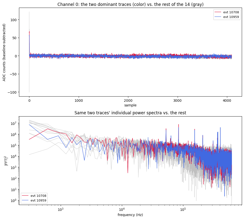
Time-domain traces and individual power spectra of events 10708 and 10959 against the other twelve traces — Events 10708 (red) and 10959 (blue) against the other 12 traces (gray). Top: baseline-subtracted time domain. Bottom: individual power spectra, log–log.

A single-sample glitch produces a broadband, roughly flat contribution to |FFT|², not narrow lines, so the leading glitch samples cannot explain these peaks.

Both traces are from Detector 1, and the lines are Detector 1’s

The 21-trace selection behind Note 3 spans Detectors 0 and 1, and the channel filter did not separate them. Of the 14 Channel 0 traces, 12 are from Detector 0 and 2 are from Detector 1: events 10708 and 10959, the two that dominate every peak.

To see whether the lines belong to those events or to the detector, the median power spectrum was taken over all quiet-baseline Channel 0 traces of each detector (bstd < 3, so pulses and drifts cannot affect a median): 908 traces from Detector 0 and 695 from Detector 1, with no further selection. The excess is each line bin’s median power divided by the median of the five bins on each side.

Line (Hz)	Detector 0	Detector 1
52,795	1.0×	50×
84,534	1.1×	181×
155,334	1.5×	58×
211,182	1.7×	27×
366,516	1.0×	16×
372,925	1.3×	20×
408,020	6.0×	28×

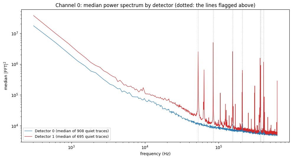
Median power spectra of Detector 0 and Detector 1 Channel 0; Detector 1 has a comb of sharp lines and a higher continuum — Median power spectrum of quiet Channel 0 traces, Detector 0 (blue, 908 traces) and Detector 1 (red, 695 traces). Dotted lines mark the seven flagged frequencies.

Detector 1 has all seven lines in its median spectrum (16–181×), so they are present in at least half of its quiet traces, and it has many more lines than the seven flagged; its continuum is also visibly higher. Detector 0 shows only the 408 kHz line, and more weakly (6×). So the sharp peaks in the 14-trace average come from its two Detector 1 traces because Detector 1 has these lines, not because those two events are unusual. It also means that averaging the two detectors together gives a spectrum that describes neither.

The 408 kHz line

The larger selections of Note 6 (192, 744 and 179 traces) are Detector 0 only, which is why the Detector 1 lines are absent there: there are no Detector 1 traces in them, so it is not a matter of dilution. The 408 kHz line is the one flagged line present in both detectors (6× in Detector 0, 28× in Detector 1). Within Detector 0, a per-trace check at the 408,020 Hz bin for the three selections gives:

Selection	Traces	Largest single trace, share of summed power	Fraction of traces > 2× local neighbors	Median excess over neighbors
`excursion_band`	192	0.03	0.73	5.3×
`excursion_band_loose`	744	0.01	0.72	4.9×
`excursion_band_AI`	179	0.03	0.72	5.1×

“Local neighbors” means the median of the five bins on each side of 408,020 Hz, taken per trace.

No trace dominates (the largest supplies 1–3%), yet about 72% of individual traces show a real excess at that exact bin, by a median factor of about 5. In the median spectrum of the 179 excursion_band_AI traces, two adjacent bins (408,020 and 408,325 Hz) stand at about 5.4–5.6×10⁴, against roughly 6–10×10³ in the bins around them — a line about two bins (~610 Hz) wide.

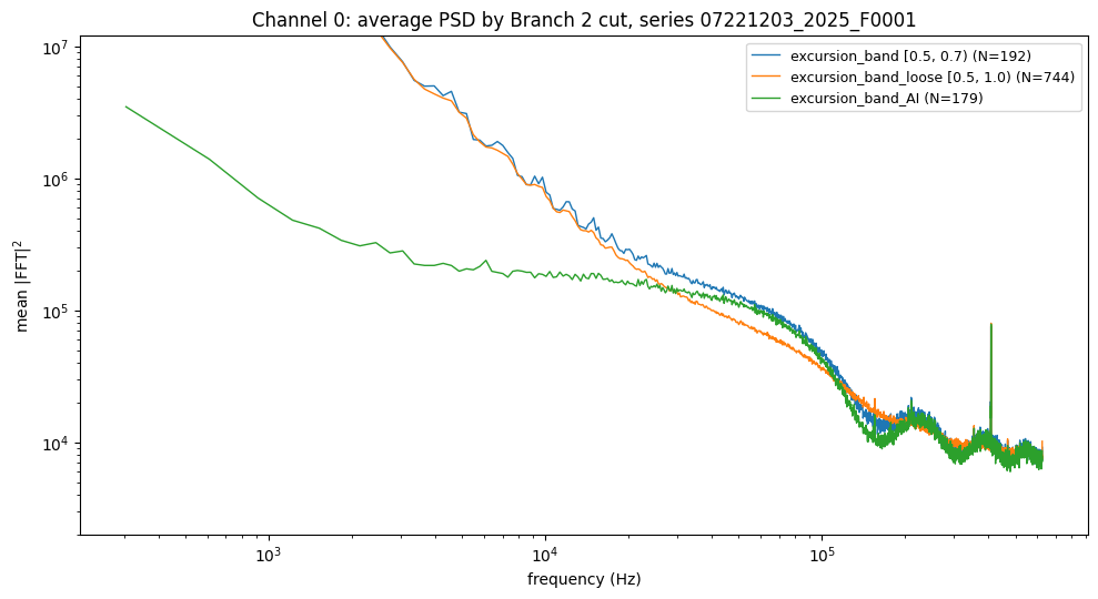
Average PSD for the three Detector 0 selections; the 408 kHz line is visible in all three — Average PSD for the three Detector 0 selections; the line near 408 kHz is visible in all of them.

Common to most traces but never dominated by one or two is what a population-wide narrowband pickup tone looks like, as opposed to per-event contamination. That it appears in both detectors, more strongly in Detector 1, suggests a source common to both readouts. The data alone cannot say what produces it (a clock, a switching supply, something in the readout); that needs the DAQ and electronics documentation.

Status / Next Steps

Identify the source of the Detector 1 line comb and of the ~408 kHz line from the electronics documentation. The comb is larger than the seven lines flagged here.
Check the other detectors and channels, the other dumps (F0002–F0005) and other series for the same lines, and whether their frequency and amplitude are stable over time.
Compute noise PSDs per detector (and per channel), not from mixed selections.
Decide how to treat the lines when a noise PSD is used for optimal filtering (mask, notch, or keep).
Build a Detector 1 noise selection with the cuts of Note 2 and Note 6 (so far only Detector 0 has been done) and repeat the peak search on it.