Noise PSD from selected traces (Channel 0, Detectors 0 and 1)
python/README.md for the evidence). What changed in this note:
- Every frequency is twice what the first version said: the bins are 305.2 Hz wide (not 152.6 Hz) and the spectrum runs up to a Nyquist frequency of 625 kHz (not 312.5 kHz).
- The frequencies quoted in the text move with it: the steep fall now starts at 305 Hz, the plateau is at 4–6 kHz and the floor starts near 200 kHz, and the sharp peaks are near 53, 85, 155, 211 and 408 kHz (not 26, 42, 78, 105 and 204 kHz).
- The figure of the average spectrum was replaced (same curve, frequency axis doubled); the time-domain overlay is in samples and is unchanged.
- Unchanged: the values of
|FFT|2(they do not depend on the sample period), the selection (21 traces, 14 on Channel 0), and every count and event number.
Superseded by: Note 6, which compares the noise PSD from larger, better-motivated selections. This note stays up for reference.
Code Repository
good_pulses_overlay.ipynb— time-domain overlay, FFT, and average power spectrum (this note); the later sections belong to Note 6 and Note 7. Pinned toeda12dc.good_noise_traces.csv— the 21-trace selection this note starts from (from the originaldump1_noise_pulses.ipynb:bstdcap 5, ratio threshold 2.45). Pinned tof03ce14.
Input: the original selection, not the 41-trace cut of Note 2
The traces come from good_noise_traces.csv, produced by the original notebook dump1_noise_pulses.ipynb. That is a different selection from the 41-trace “first cut” of Note 2, and the two share no events:
| Original selection (this note) | First cut of Note 2 | |
|---|---|---|
| Notebook | dump1_noise_pulses.ipynb | 07221203_2025_dump1_noise.ipynb |
| Scope | all detectors, all four channels of dump F0001 | Detector 0 / Channel 0 only (1517 traces) |
| Quiet baseline | bstd < 5 (absolute) | bstd < 32.48 (its own 75th percentile) |
| Excursion | ratio < 2.45 (the notebook’s 25th percentile over all channels) | ratio < 1.93 (its own 25th percentile) |
Leading glitch samples in bstd | included | first 10 skipped |
| Traces kept | 21 (Detector 0: 12 on channel 0, 2 on channel 1, 4 on channel 3; Detector 1: 2 on channel 0, 1 on channel 3) | 41 |
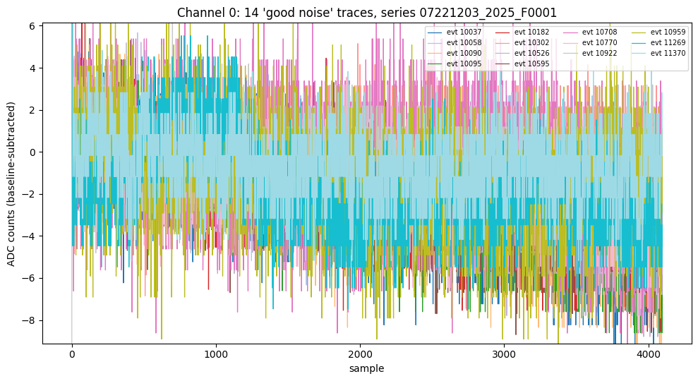
Restricting the 21 traces to Channel 0, the best-represented channel, leaves 14: 12 from Detector 0 and 2 from Detector 1 (events 10708 and 10959). The channel filter did not separate the detectors, so this PSD mixes two detectors. Note 7 shows why that matters.
Why the two selections do not overlap
Applying the original cut to Detector 0 / Channel 0 alone gives 12 traces, none among the 41. All 12 are quiet baselines: with the first 10 samples skipped, as in Note 2, their bstd is a median of 1.56 (3.84 as originally computed) and their ratio is 3.3–6.1 (1.6–2.4 as originally computed). That places them in the broad hump of log10(ratio) 0.5–1.0 of Note 2 (here 0.52–0.79). Note 2’s first cut instead requires ratio < 1.93, which selects the contaminated near-zero spike, so the two cuts pick out different populations.
The original cut also has a selection bias. Its low ratio comes from a bstd inflated by the leading samples. Among the 868 quiet Detector 0 / Channel 0 traces (bstd < 2.5 with the glitch skipped), 160 have an original bstd more than 1.3× the glitch-skipped value and 708 do not. The original cut kept 12 of the 160 and none of the 708: it selects quiet traces whose leading samples inflate bstd, and systematically excludes equally quiet traces without that. (All of this is computed in the last section of good_pulses_overlay.ipynb.)
Time domain
Each trace is baseline-subtracted with the mean of its own pretrigger window. A couple of the traces have a single-sample startup transient in the first few dozen samples, a known quirk of this digitizer data rather than a real pulse. The plot’s y-axis is clipped to the 0.5–99.5 percentile of all plotted samples so the transient does not wash out the noise texture.
Frequency domain
The real FFT (np.fft.rfft) is taken of every trace. The sample period is 0.8 µs (1.25 MHz sample rate; the first version of this note used 1.6 µs, which was wrong), so with 4096 samples per trace the bins are 305.2 Hz wide and run up to the 625 kHz Nyquist frequency. The power spectrum is spectrum × conj(spectrum) (its imaginary part is zero by construction), plotted log–log with the DC bin dropped. Averaging the 14 spectra bin by bin gives a first noise PSD estimate:
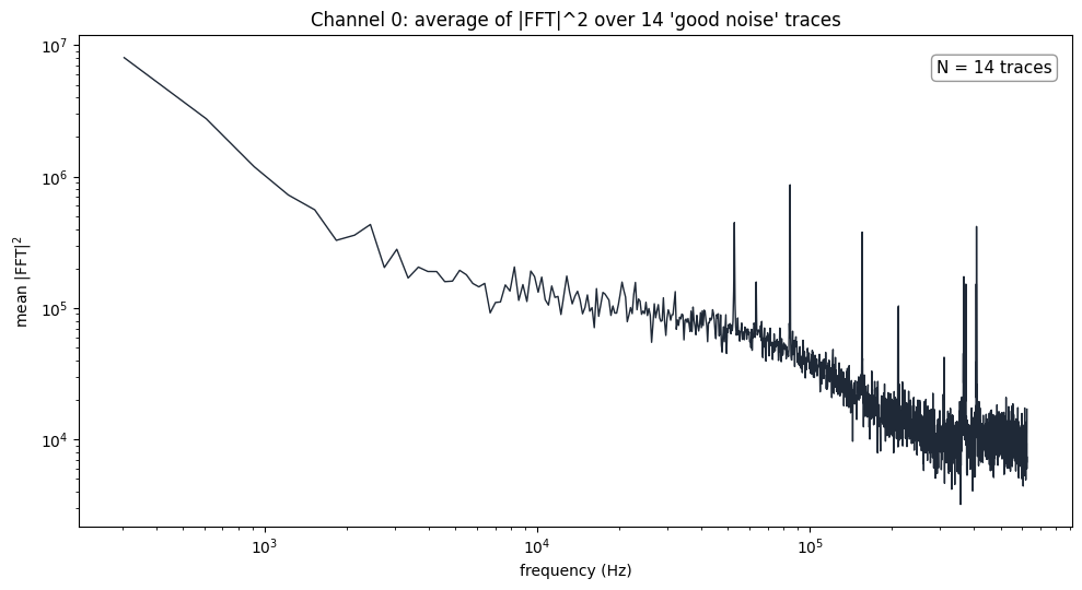
|FFT|2 over the 14 traces, log–log, real Hz.The average falls steeply from about 8×10⁶ at 305 Hz (the first bin) to ~2×10⁵ near 4–6 kHz, declines slowly out to ~40 kHz, then rolls off to a floor near 104 above ~200 kHz. Several sharp peaks (near 53, 85, 155, 211 and 408 kHz, among others) sit on top of it. Where those peaks come from is the subject of Note 7.
Conventions and caveats
- The plotted quantity is the raw NumPy
|FFT|2, not a normalized one-sided PSD in units per Hz. Golwala’s SLAC thesis (Appendix B, “Noise and Optimal Filtering”) puts a1/Non the forward transform, opposite to NumPy, so the absolute scale here is not directly comparable to it. - The leading glitch samples are kept in the traces that go into the FFT. Baseline subtraction skips them only when computing the mean it subtracts; it does not remove them. This was a deliberate choice.
- The selection is small (14 traces), mixes two detectors, and is biased toward quiet traces with glitch-inflated
bstd(see above). The sharp peaks in the average come from its two Detector 1 traces (Note 7).
Status / Next Steps
- Done since: the PSD from the larger, better-motivated selections of Note 2 is compared in Note 6.
- Compute the PSD per detector instead of mixing them; Note 7 shows the two detectors’ spectra differ.
- Repeat for the other channels; Channel 2 never passed the original cut.
- Normalize to a proper one-sided PSD following the thesis convention before using it for optimal filtering.